Plotting Curves and Points, Least-Squares Example
Lisa Oberbroeckling
Spring 2011
Contents
NOTE: m-files don't view well in Internet Explorer. Use Mozilla Firefox or Safari instead to view these pages.
You should always have the following commands at the top to "start fresh"
clear
clf     % New (to you): clears the figure window
format
clc
Basic Plot Example
There are several ways to plot data points and plot curves. I will show you one of the ways.
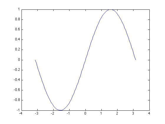
The basic plot command is plot(x,y) where x and y are vectors. This would plot the curve connecting the points that x,y make up. Here is an example:
x1 = linspace(-pi,pi);      % creating a vector of 100 values from -pi to pi
y1 = sin(x1);               % creating the y's for these x values
plot(x1,y1)
Plotting Data Points
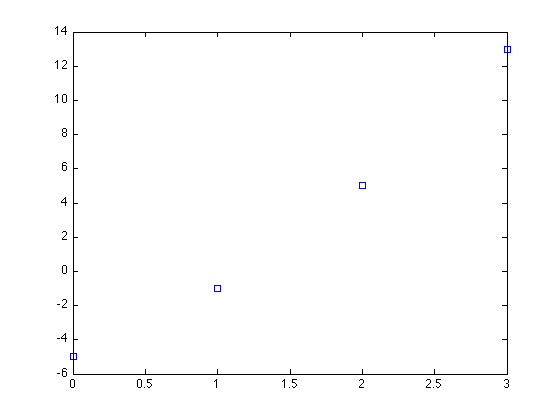
If we wanted to plot data points, we'd specify "markers". Here's an example:
x2 = [0 1 2 3];
y2 = x2.^2 + 3*x2 - 5;      % Notice the .^: this is for component-wise calculations
plot(x2,y2,'s')             % s for square
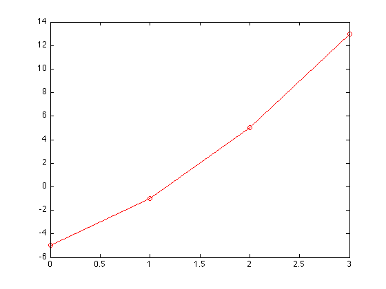
If we wanted to connect the points, we'd specify the line type along with the marker type:
plot(x2,y2,'o-r') % o is for circle, - is for solid line, r is for red
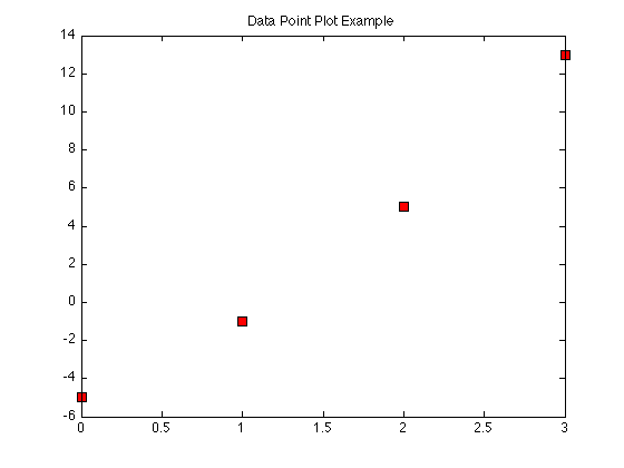
We can increase the size of the markers and specify a marker face and marker edge color (r is for red, k is for black). A title is also added to the figure.
plot(x2,y2,'s','MarkerSize',7,'MarkerFaceColor','r','MarkerEdgeColor','k')
title('Data Point Plot Example')
Plotting Multiple Curves and/or Data Points in Same Figure
Normally, each plot command replaces the previous plot command so that you'd only see the latest plot. The hold on command allow you to add plot commands to the existing figure until you type the command hold off.
x3 = linspace(-5,5);
y3 = 1/5*x3.^2;
plot(x3,y3)
y4 = cos(x3);
hold on
plot(x3,y4, 'g--', 'LineWidth',2)      % specifies green dashed plot and makes the lines thicker
a=[0 2 -3 5];
b=[-1 3 2 1];
plot(a,b,'o','MarkerSize',7,'MarkerFaceColor','r','MarkerEdgeColor','k')
hold off
title('Example of multiple plots on one figure')
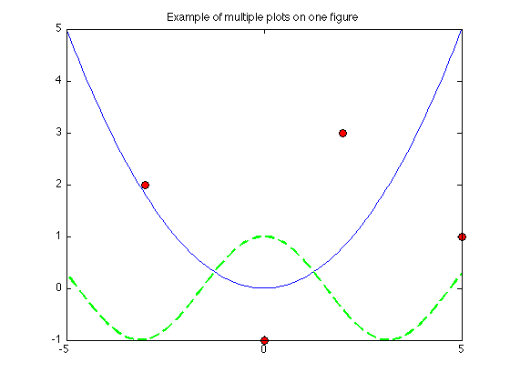
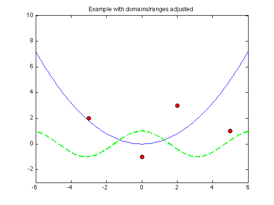
The next example is the same as above except that adjusts the domain for x3 and specifies the x and y ranges in the figure for better viewing:
x3 = linspace(-6,6);
y3 = 1/5*x3.^2;
plot(x3,y3)
y4 = cos(x3);
hold on
plot(x3,y4, 'g--', 'LineWidth',2)      % specifies green dashed plot and makes the lines thicker
a=[0 2 -3 5];
b=[-1 3 2 1];
plot(a,b,'o','MarkerSize',7,'MarkerFaceColor','r','MarkerEdgeColor','k')
title('Example with domains/ranges adjusted')
xlim([-6,6])
ylim([-3,10])
hold off
Least Squares Solutions
Section 6.4 of the textbook discusses a very important idea called least-squares solutions. Both in this section and the MATLAB appendices, several ways to have MATLAB to fit data to a curve are shown (specically, fitting to a polynomial). The book even discusses using a special function written by the textbook authors that can be downloaded. I will show you the two basic (main) ways to do find a least-squares solution in MATLAB without the use of special functions or special data fitting commands.
Consider the following system of equations:


If we try and solve this system  , the system is overdetermined and has no solution:
A=[1 1;-1 1;2 3];
b = [6;3;9];
B = [A b]
rref(B)     % putting augmented matrix in REF
B =

     1     1     6
    -1     1     3
     2     3     9


ans =

     1     0     0
     0     1     0
     0     0     1
We want to find the least squares solution which would give the best approximation to a solution. The first way of a least-squares solution  for an overdetermined system is by "left-division". For this you just type A\b.
A=[1 1;-1 1;2 3]
b = [6;3;9]
xstar = A\b
A =

     1     1
    -1     1
     2     3


b =

     6
     3
     9


xstar =

    0.5000
    3.0000
The other way is to find the pseudoinverse of  using the command pinv(A), and multiply this (on the right) by
  , just as you would if inv(A) existed. The text discusses the Moore-Penrose pseudoinverse in more detail than what is here.
xstar2 = pinv(A)*b
xstar2 =

    0.5000
    3.0000
Notice you get the same answer. This is true for overdetermined systems, and if you don't need the pseudoinverse computed for any other reason, the left division computation of the least-squares solution is actually more efficient (although for our examples efficiency is not an issue).
Data Fitting with Least Squares
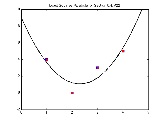
I will do Problem 22 from section 6.4 in the text as an example.
We want to fit the following data points to a parabola  .
.
I'm using the variable  in the polynomial so it doesn't become confusing with our vector
  that is used in the equation .
By plugging in the x-values of the data points, we get the following equations


Our system then becomes and we want to solve for which is the vector of our coefficents  but the system is overdetermined so we find the least-squares solution :
A = [1 1 1;4 2 1; 9 3 1;16 4 1]
b = [4;0;3;5]
xstar = A\b
rats(xstar)
A =

     1     1     1
     4     2     1
     9     3     1
    16     4     1


b =

     4
     0
     3
     5


xstar =

    1.5000
   -6.9000
    9.0000


ans =

      3/2
    -69/10
       9
Thus the least-squares solution is
![$$ x^* = \left[\begin{array}{r} 3/2 \\ -69/10 \\ 9 \end{array}\right] $$](PlotLeastSquaresExample1_eq66286.png)
so our least-squares parabola is:
We now plot it:
x = [1 2 3 4];                  % x-values of the data points
y = [4 0 3 5];                  % y-values of the data points
t = linspace(0,5);              % domain for curve
p = 3/2*t.^2 - 69/10*t + 9;     % p for polynomial since y was taken
plot(t,p,'k','LineWidth',2)
hold on
plot(x,y,'s','MarkerSize',7,'MarkerFaceColor','r','MarkerEdgeColor','b')
title('Least Squares Parabola for Section 6.4, #22')
ylim([-2,10])
hold off
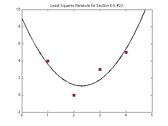
Another way
For the above example, instead of typing in the matrix A by hand, we could notice the pattern each row of A would have. I'm clearing the variables to "start fresh" to show you how you can get the same A and b as above by just plugging in the data points by hand and doing some calculations on them.
clear
x=[1;2;3;4];
y=[4;0;3;5];    % notice both x and y are column vectors
c = ones(4,1);   % creates a column vector of all ones
A = [x.^2 x c]
xstar = A\y
A =

     1     1     1
     4     2     1
     9     3     1
    16     4     1


xstar =

    1.5000
   -6.9000
    9.0000
We can even define the polynomial without typing in the coefficients by hand:
t=linspace(0,5);
a=xstar(1);
b=xstar(2);
c=xstar(3);
p = a*t.^2 + b*t + c;
plot(t,p,'k','LineWidth',2)
hold on
plot(x,y,'s','MarkerSize',7,'MarkerFaceColor','r','MarkerEdgeColor','b')
title('Least Squares Parabola for Section 6.4, #22')
ylim([-2,10])
hold off
Be aware that there are built-in polynomial and data-fitting commands in MATLAB but we are not using any of them so as to not overwhelm you.