Plotting Vector Functions (Space Curves)
Lisa Oberbroeckling, Fall 2015
Contents
NOTE: m-files don't view well in Internet Explorer. Use Mozilla Firefox or Safari instead to view these pages.
You should always have the following commands at the top to "start fresh"
clc, clf    % clears the command window and figure window
clear       % clears ALL variables
format      % resets the format to the default format
Example 1 (2D example)
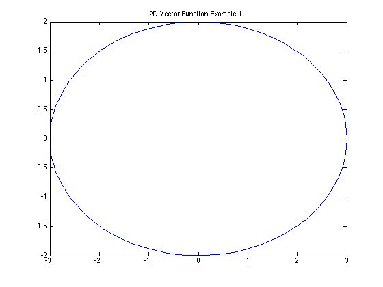
In 2D, vector functions are no different than the parametric equations you saw in Chapter 10 in Calculus.
To plot them, you must first establish your domain for \( t \). The easiest way to do this is with the command LINSPACE.
t = linspace(0,2*pi);
IMPORTANT: notice the semi-colon at the end of these lines; if there is none, all of those values for \( t \)(and \( x\), \( y\), etc. below) will appear in your command window.
Now we enter the equations for \( x \) and \( y\), using component-wise calculations.
x = 3*cos(t);
y = 2*sin(t);
Now we can plot the x and y values. For 2D plots, it's simple:
plot(x,y)
title('2D Vector Function Example 1')
Example 2 (2D example)
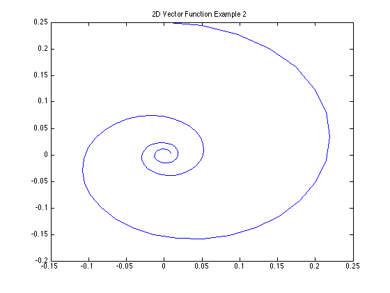
The above equations didn't need component-wise calculations. This example does: \( \vec{r}(t) = \left\langle \dfrac{\sin(2t)}{4+t^2}, \dfrac{\cos(2t)}{4+t^2}\right\rangle\)
t = linspace(0,10);
x = sin(2*t)./(4 + t.^2);
y = cos(2*t)./(4 + t.^2);
plot(x,y)
title('2D Vector Function Example 2')
Example 3 (3D example)
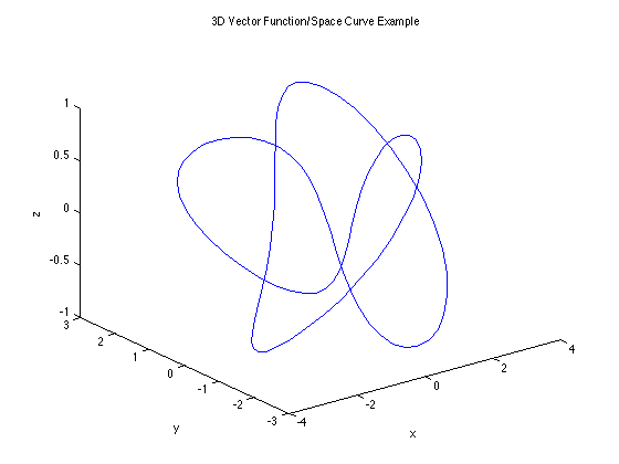
This example involves component-wise calculations, and the domain needed to be adjusted to show the entire trefoil knot.
Notice for a 3D space curve, the command is PLOT3 instead of PLOT.
It is always good to label the axes for perspective.
t=linspace(0,4*pi);
x=(2+cos(1.5*t)).*cos(t);
y=(2+cos(1.5*t)).*sin(t);
z=sin(1.5*t);
plot3(x,y,z)
xlabel('x'), ylabel('y'), zlabel('z')
title('3D Vector Function/Space Curve Example')
Example 4 (bad domain example)
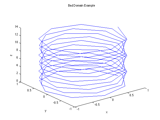
The following is an example in thich the domain doesn't have enough points and it creates a jagged curve that should be smooth.
t=linspace(0,4*pi);
x=cos(6*t);
y=sin(6*t);
z=t;
plot3(x,y,z)
xlabel('x'), ylabel('y'), zlabel('z')
title('Bad Domain Example')
Example 3c (better domain)
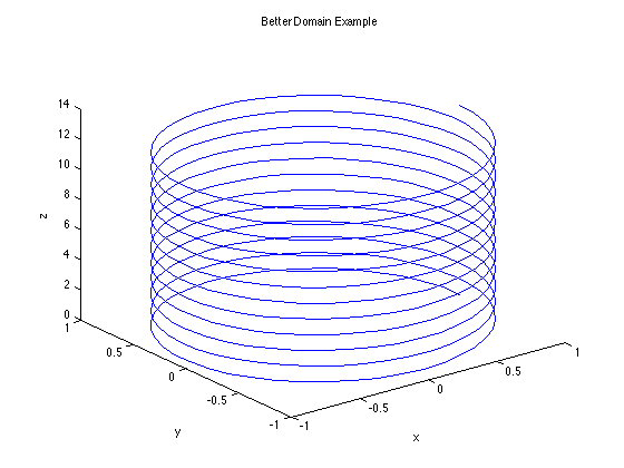
The problem above was because by default the linspace(a,b) command creates one hundred values between a and b for MATLAB use to connect to plot the graph. By having linspace(a,b,n), you are specifying n values between a and b. So below, we have t be a vector of 500 values between 0 and 4pi with which to create the x,y, and z values to build points to connect into a graph.
t=linspace(0,4*pi,500);
x=cos(6*t);
y=sin(6*t);
z=t;
plot3(x,y,z)
xlabel('x'), ylabel('y'), zlabel('z')
title('Better Domain Example')
Example 5 (adjusting view)
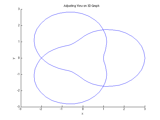
You can adjust the view. Using this command may involve experimentation with the values and rerunning the script.
t=linspace(0,4*pi);
x=(2+cos(1.5*t)).*cos(t);
y=(2+cos(1.5*t)).*sin(t);
z=sin(1.5*t);
plot3(x,y,z)
view(0,90)
xlabel('x'), ylabel('y'), zlabel('z')
title('Adjusting View on 3D Graph')
Example 6 (Sphere Command)
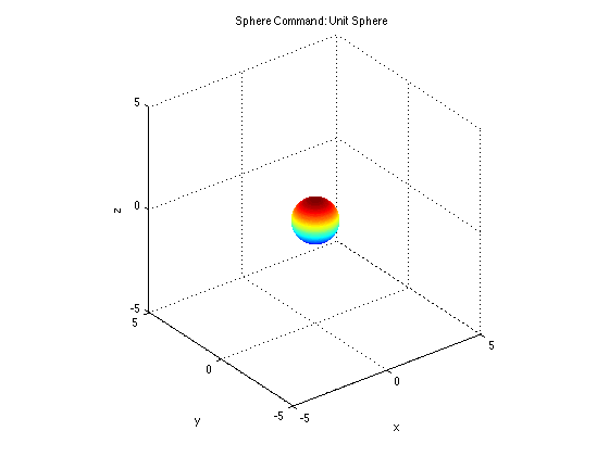
The SPHERE command will set up variables x, y, and z to form a unit sphere using the surf or mesh commands. Without going into details, here are examples
[x,y,z]=sphere(100);
mesh(x,y,z)
xlabel('x'), ylabel('y'), zlabel('z')
title('Sphere Command: Unit Sphere')
axis equal
axis([-5 5 -5 5 -5 5])
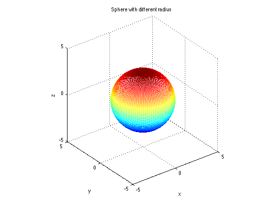
How to get one of a different radius (\( r=3 \)) than 1:
[x,y,z]=sphere(100);
mesh(3*x,3*y,3*z)
xlabel('x'), ylabel('y'), zlabel('z')
title('Sphere with different radius')
axis equal
axis([-5 5 -5 5 -5 5])
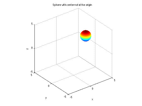
How to get a sphere with a different center \( C(2,-1,3) \) than the origin:
[x,y,z]=sphere(100);
mesh(x+2,y-1,z+3)
xlabel('x'), ylabel('y'), zlabel('z')
title('Sphere with center not at the origin')
axis equal
axis([-5 5 -5 5 -5 5])
QUESTION: How could you get ANY sphere - different center than origin and radius other than 2?
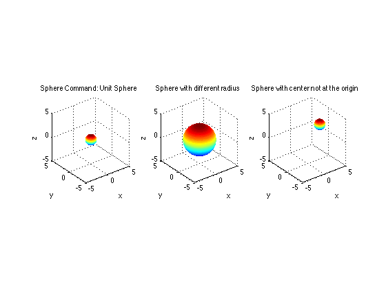
Here they are side-by-side for comparison
subplot(131)
mesh(x,y,z)
xlabel('x'), ylabel('y'), zlabel('z')
title('Sphere Command: Unit Sphere')
axis equal
axis([-5 5 -5 5 -5 5])
subplot(132)
mesh(3*x,3*y,3*z)
xlabel('x'), ylabel('y'), zlabel('z')
title('Sphere with different radius')
axis equal
axis([-5 5 -5 5 -5 5])
subplot(133)
mesh(x+2,y-1,z+3)
xlabel('x'), ylabel('y'), zlabel('z')
title('Sphere with center not at the origin')
axis equal
axis([-5 5 -5 5 -5 5])
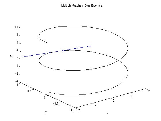
Example 7 (Multiple Plots on One Figure)
You must huse the hold on and hold off commands around the additional plot/plot3/mesh, etc. commands for all to show up within the same figure.
clf
t = linspace(-pi,3*pi);
x = 2*cos(t);
y = sin(t);
z = t;
plot3(x,y,z, 'k')
xlabel('x'), ylabel('y'), zlabel('z')
title('Multiple Graphs in One Example')
hold on         % use this to add more plots to current figure
t2 = linspace(-1,1);
x2=-2*t2;
y2=1 + 0*t2;
z2=pi/2 + t2;
plot3(x2,y2,z2)
hold off         % make sure you have this at the end
