2D Graphs
L. Oberbroeckling, Fall 2011.
NOTE: m-files don't view well in Internet Explorer. Use Mozilla Firefox or Safari instead to view these pages.
Contents
You may want to have the following commands at the top of your script files to "start fresh"
clc         % clears the command window
clear       % clears ALL variables
format      % resets the format to the default format
There are many other examples on the H-drive!
There are several ways to produce graphs of functions. This page will not show all of them; it will show the way that is the most customizable and can be easily extended to more complicated settings (like parametric equations, 3D, etc.) This is also a learn-by-example page. I do not explain every command or show everything. It is up to you to experiment and look up these commands to better understand them.
- Set up your domain by creating a vector x (or whatever variable name you want as long as it starts with a letter). There are several ways to do this, the easiest is using the command linspace:
- x=linspace(a,b) will create a vector called x with 100 components comprised of equally spaced (linearly spaced) numbers from a to b.
- x=linspace(a,b,n) will create a vector called x with n components comprised of linearly spaced numbers from a to b.
- Calculate the y-values for x USING COMPONENT-WISE COMPUTATIONS
- IMPORTANT TIP: make sure you use ; at the end of the lines defining your variables so you don't get extraneous output (see "Forgetting Semi-colons" below).
- Basic plot command: plot(x,y)
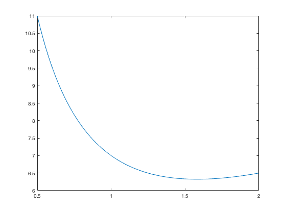
Basic 2D Graph
x=linspace(0.5,2);
y= (2*x.^2 + 5)./x;
plot(x,y)
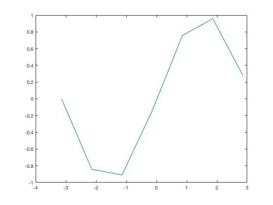
Bad Domain Definition
This example shows how you need to be careful when defining x.
x=-pi:pi;
y=sin(x);
plot(x,y)
Better Domain
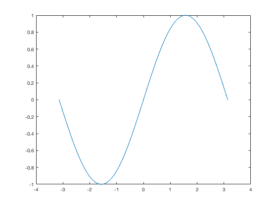
The way is defined above, x is vector of numbers starting at -pi, increasing by 1 and ending at pi (or in this case, 2.8584 because that is the biggest number less than pi in the sequence). Thus the graph is a bunch of lines connecting these points, and so y=sin x appears jagged. Here's a better way:
x2=-pi:.1:pi;
y=sin(x2);
plot(x2,y)
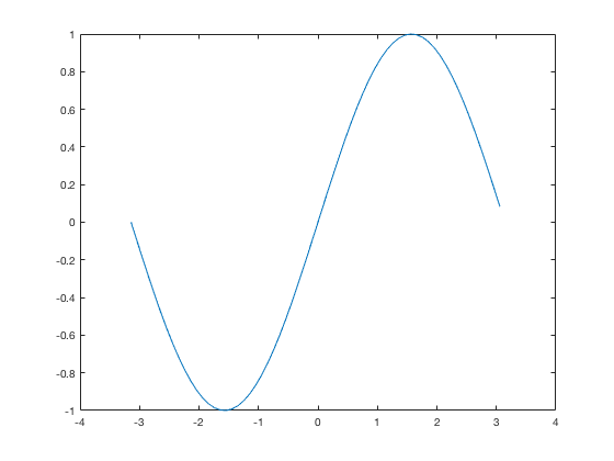
The way x2 is defined above, it is a vector of numbers between -pi and pi with an increment of .1. You may need to experiment with this increment depending on what your curve is to get a smooth graph but without too many elements in the vector so the computer isn't unnecessarily slow. Using linspace instead (as mentioned above) is many times easier.
x3=linspace(-pi,pi);
y=sin(x3);
plot(x3,y)
Forgetting Semi-colons
Here is why you want to use semi-colons:
x3=linspace(-pi,pi)
y=sin(x3)
plot(x3,y)
x3 =

  Columns 1 through 7

   -3.1416   -3.0781   -3.0147   -2.9512   -2.8877   -2.8243   -2.7608

  Columns 8 through 14

   -2.6973   -2.6339   -2.5704   -2.5069   -2.4435   -2.3800   -2.3165

  Columns 15 through 21

   -2.2531   -2.1896   -2.1261   -2.0627   -1.9992   -1.9357   -1.8723

  Columns 22 through 28

   -1.8088   -1.7453   -1.6819   -1.6184   -1.5549   -1.4915   -1.4280

  Columns 29 through 35

   -1.3645   -1.3011   -1.2376   -1.1741   -1.1107   -1.0472   -0.9837

  Columns 36 through 42

   -0.9203   -0.8568   -0.7933   -0.7299   -0.6664   -0.6029   -0.5395

  Columns 43 through 49

   -0.4760   -0.4125   -0.3491   -0.2856   -0.2221   -0.1587   -0.0952

  Columns 50 through 56

   -0.0317    0.0317    0.0952    0.1587    0.2221    0.2856    0.3491

  Columns 57 through 63

    0.4125    0.4760    0.5395    0.6029    0.6664    0.7299    0.7933

  Columns 64 through 70

    0.8568    0.9203    0.9837    1.0472    1.1107    1.1741    1.2376

  Columns 71 through 77

    1.3011    1.3645    1.4280    1.4915    1.5549    1.6184    1.6819

  Columns 78 through 84

    1.7453    1.8088    1.8723    1.9357    1.9992    2.0627    2.1261

  Columns 85 through 91

    2.1896    2.2531    2.3165    2.3800    2.4435    2.5069    2.5704

  Columns 92 through 98

    2.6339    2.6973    2.7608    2.8243    2.8877    2.9512    3.0147

  Columns 99 through 100

    3.0781    3.1416


y =

  Columns 1 through 7

   -0.0000   -0.0634   -0.1266   -0.1893   -0.2511   -0.3120   -0.3717

  Columns 8 through 14

   -0.4298   -0.4862   -0.5406   -0.5929   -0.6428   -0.6901   -0.7346

  Columns 15 through 21

   -0.7761   -0.8146   -0.8497   -0.8815   -0.9096   -0.9341   -0.9549

  Columns 22 through 28

   -0.9718   -0.9848   -0.9938   -0.9989   -0.9999   -0.9969   -0.9898

  Columns 29 through 35

   -0.9788   -0.9638   -0.9450   -0.9224   -0.8960   -0.8660   -0.8326

  Columns 36 through 42

   -0.7958   -0.7557   -0.7127   -0.6668   -0.6182   -0.5671   -0.5137

  Columns 43 through 49

   -0.4582   -0.4009   -0.3420   -0.2817   -0.2203   -0.1580   -0.0951

  Columns 50 through 56

   -0.0317    0.0317    0.0951    0.1580    0.2203    0.2817    0.3420

  Columns 57 through 63

    0.4009    0.4582    0.5137    0.5671    0.6182    0.6668    0.7127

  Columns 64 through 70

    0.7557    0.7958    0.8326    0.8660    0.8960    0.9224    0.9450

  Columns 71 through 77

    0.9638    0.9788    0.9898    0.9969    0.9999    0.9989    0.9938

  Columns 78 through 84

    0.9848    0.9718    0.9549    0.9341    0.9096    0.8815    0.8497

  Columns 85 through 91

    0.8146    0.7761    0.7346    0.6901    0.6428    0.5929    0.5406

  Columns 92 through 98

    0.4862    0.4298    0.3717    0.3120    0.2511    0.1893    0.1266

  Columns 99 through 100

    0.0634    0.0000

Clearly we don't need to see the values of x and y; we just want their points connected to make a nice graph.
Multiple Graphs in 2D
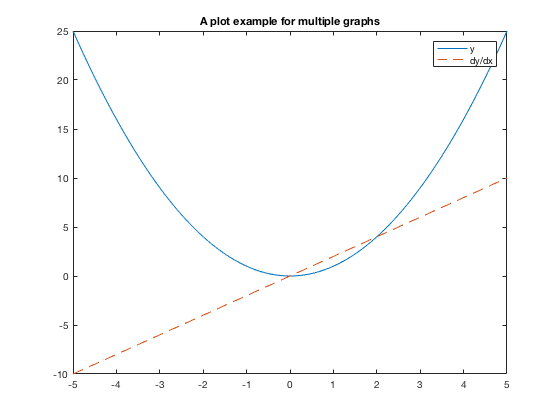
Here's another basic example. This shows you one way to put 2 functions on the same graph with different colors and line types, along with a legend and title.
clear
x=linspace(-5,5);
y1=x.^2;          % y values of the first plot
y2 = 2*x;         % y values of the second plot
plot(x,y1,'-', x,y2,'--')
legend('y','dy/dx')
title('A plot example for multiple graphs')

Multiple Graphs using HOLD ON/HOLD OFF
The above plot command can get cumbersome if you have a lot of functions to plot or a lot of fine-tuning of the colors, line types, etc. If you experiment, you'll notice that if you follow a plot command with another plot command, the figure will only show the last plot command. If you use the hold on command, any command that has anything to do with plotting will appear on the current figure. Even subsequent plot commands will just add to the current figure. Thus it is very important to use the hold off command when done.
clear
x=linspace(-5,5);
y1=x.^2;          % y values of the first plot
y2 = 2*x;         % y values of the second plot
plot(x,y1)
hold on
plot(x,y2,'--')
legend('y','dy/dx')
title('A plot example for multiple graphs')
hold off            % VERY IMPORTANT TO HAVE THE HOLD OFF COMMAND!
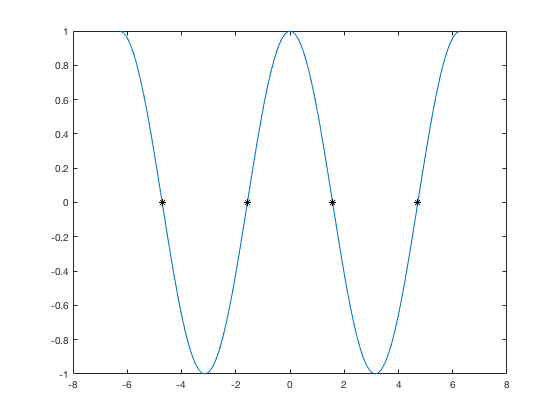
Plotting Points
You must specify that you don't want the points "connected" by specifying a marker. There are several types of markers.
clear
x = linspace(-2*pi, 2*pi);
y = cos(x);
x2 = [-3*pi/2, -pi/2, pi/2, 3*pi/2];
y2=cos(x2);
plot(x,y)
hold on
plot(x2,y2,'*k')
hold off
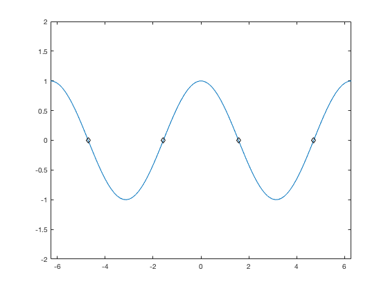
Setting Axes Ranges
Sometimes we'd like to adjust the x-values and/or y-values shown.
plot(x,y)
hold on
plot(x2,y2,'dk')
hold off
xlim([-2*pi,2*pi])
ylim([-2,2])
Graphing Lines
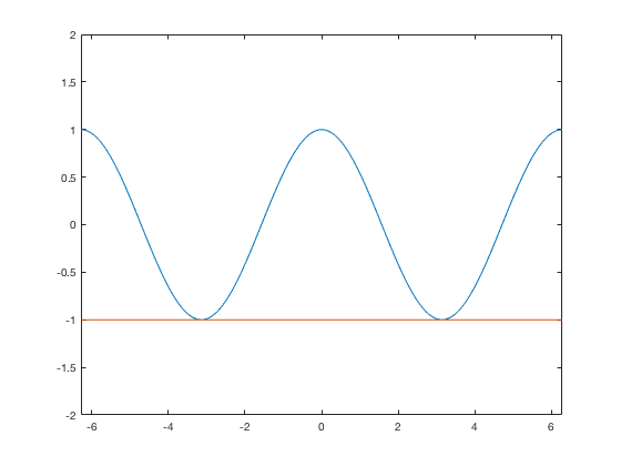
For the horizontal line y=1, it doesn't work to just define y=3. You need a y-value of 3 for every x-value in the domain. Thus you can do something like this:
y3=0*x + -1;
plot(x,y,x,y3)
axis([-2*pi,2*pi, -2, 2])
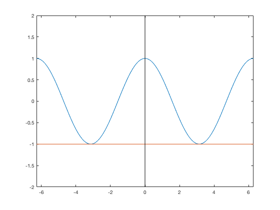
Similarly, you can do it for a vertical line, but for every y-value, define an x-value. You may need to adjust your y-values to get it to work nicely.
yv= -2:2;
xv = 0*yv + 0;
plot(x,y,x,y3,xv,yv,'k')
axis([-2*pi,2*pi, -2, 2])
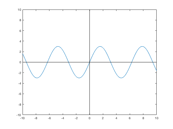
Or you can have lines be defined by points and connect them (with or without markers).
clear
x=linspace(-10,10);
xvalues = [-10,10];
yvalues = [0,0];
plot(x,3*sin(x),xvalues,yvalues,'k',yvalues,xvalues, 'k')
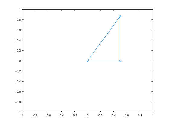
plot([0,1/2,1/2,0],[0,0,sqrt(3)/2,0],'-o')
axis([-1,1,-1,1])