Plotting 3D Surfaces

L. Oberbroeckling, Fall 2014.

This has a lot of stuff; read the contents carefully!

NOTE: m-files don't view well in Internet Explorer. Use Mozilla Firefox or Safari instead to view these pages.

Contents

You may want to have the following commands at the top of your script files to "start fresh"

clc         % clears the command window
clear       % clears ALL variables
format      % resets the format to the default format

There are many other examples on the H-drive!

There are several ways to produce graphs of functions. This page will not show all of them; it will show the way that is the most customizable and can be easily extended to more complicated settings (like parametric equations, 3D, etc.) This is also a learn-by-example page. I do not explain every command or show everything. It is up to you to experiment and look up these commands to better understand them.

Basic steps

There are 4 main steps:

Basic 3D Surface Example using SURF

This example shows one way to plot 3D surfaces. The meshgrid command is vital for 3D surfaces!

Defining the domain here is even trickier than for 2D. You don't want too few points in the "grid" or it will appear jagged, but too many and the computer will slow down or even hang!

xd=linspace(-1,1);
yd=linspace(0,2*pi);
[x,y]=meshgrid(xd,yd);
z=x.*cos(y);
surf(x,y,z)

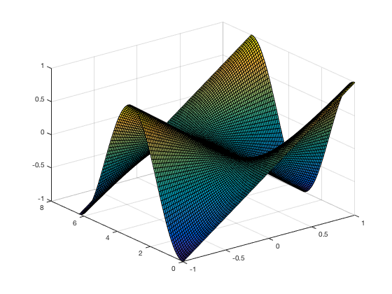
Using MESH

We could have equally used the following command

mesh(x,y,z)        % check out the difference in the graphs!

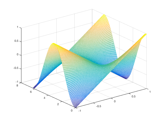
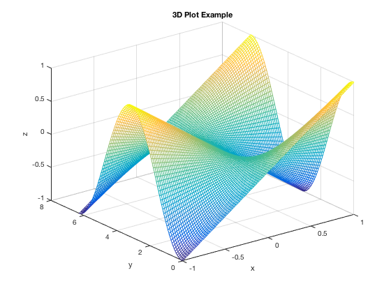
Adding axes labels, titles

CAREFUL! One of mesh and surf may be more appropriate for different graphs

Following labels the axes and creates a title

mesh(x,y,z)
xlabel('x'),ylabel('y'),zlabel('z')
title('3D Plot Example')

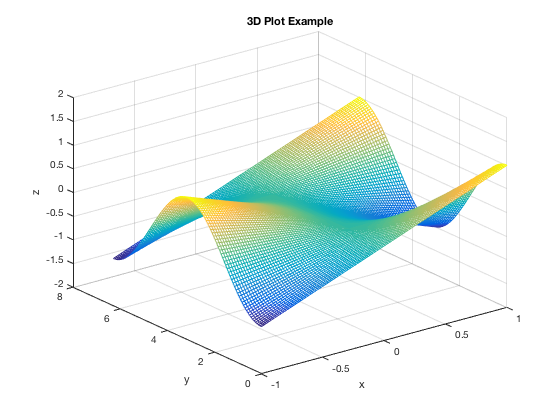
Limiting axes ranges

The ZLIM command changes the range of the z-axis shown (you can likewise use XLIM and/or YLIM).

mesh(x,y,z)
zlim([-2,2])
xlabel('x'),ylabel('y'),zlabel('z')
title('3D Plot Example')

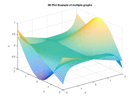
Multiple 3D Surfaces

This example demonstrates how to plot more than one graph on the same figure. Notice in this example we used a different way to get the domain for x,y using linspace as opposed to the above example. Again, you may need to adjust how many points are used to make the graph not too jagged (if number too low) or not hang the computer (number too high).

[x,y]=meshgrid(linspace(-2,2));
z1=y.*exp(x.^2-5);
mesh(x,y,z1)
xlabel('x'),ylabel('y'),zlabel('z')
title('3D Plot Example of multiple graphs')
hold on
z2=1/2*x.*cos(y);
mesh(x,y,z2)
hold off    %%%%% DON'T FORGET TO HOLD OFF!! %%%%%

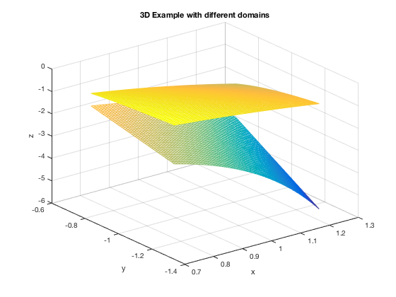
Another 3D Surface Example

This example demonstrates a way to have different x and y ranges. The command linspace(a,b,N) gives N points between a and b so linespace(0.75,1.25,81) gives 51 points between 0.75 and 1.25. The number of points used for x and y MUST BE EQUAL thus, 51 for both of them in this example CAREFUL! this "51" number may need to be adjusted to make a smooth, nice graph and not hang the computer

u=linspace(0.75,1.25,51);
v=linspace(-1.25,-0.75,51);
[x,y]=meshgrid(u,v);
z1=y.*exp(x.^2);
mesh(x,y,z1)
xlabel('x'),ylabel('y'),zlabel('z')
title('3D Example with different domains')
hold on
z2=x.^2./y;
mesh(x,y,z2)
hold off

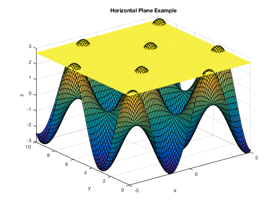
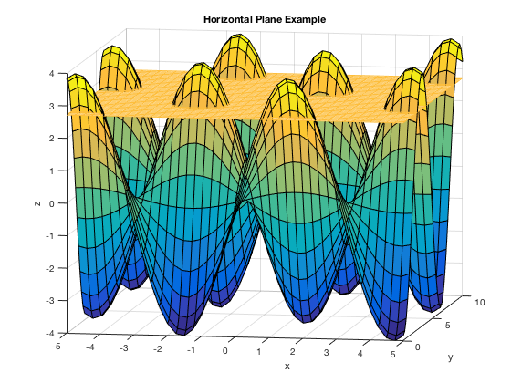
Graphing a Horizontal Plane

This example shows how to graph a horizontal plane. If you were to just define \( z = e \), it would only assign z to be one number, but we need the number e assigned at the z-value for each (x,y) in the domain. thus, you can do the following:

u=linspace(-5,5,81);
v=linspace(0,10,81);
[x,y]=meshgrid(u,v);
z1=3*sin(x).*cos(y);
surf(x,y,z1)
xlabel('x'),ylabel('y'),zlabel('z')
title('Horizontal Plane Example')
hold on
z2=0*x + exp(1);    % the 0*x + exp(1) makes sure the output for z2 is the same size
                    % as x and y, but only has the value of e in each component.
mesh(x,y,z2)
hold off

Adjusting view and the meshgrid size

Same graph as above, but adjusting the view and the number of points in the meshgrid

u=linspace(-5,5,41);
v=linspace(0,10,41);
[x,y]=meshgrid(u,v);
z1=4*sin(x).*cos(y);
surf(x,y,z1)
xlabel('x'),ylabel('y'),zlabel('z')
title('Horizontal Plane Example')
hold on
z2=0*x + exp(1);    % the 0*x + exp(1) makes sure the output for z2 is the same size
                    % as x and y, but only has the value of e in each component.
mesh(x,y,z2)
view(10,10)
hold off

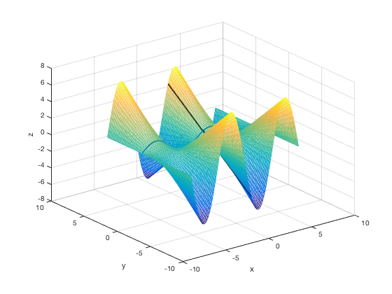
Combining vector functions and surfaces

You can plot surfaces and vector functions on the same figure using the hold on command.

[x,y]=meshgrid(linspace(-2*pi,2*pi));
z=y.*sin(x);
mesh(x,y,z)
hold on
t=linspace(-2*pi,2*pi);
X=t;
Y=1+0*t;
Z=sin(t);
X2=pi/4+0*t;
Y2=t;
Z2=sqrt(2)/2*t;
plot3(X,Y,Z,'LineWidth',2)
plot3(X2,Y2,Z2,'k','LineWidth',2)
hold off
xlabel('x'),ylabel('y'),zlabel('z')

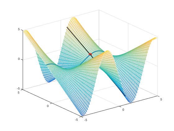
Plotting Points

As in the 2D case, just add points using plot3 command and specifying the marker type.

mesh(x,y,z)
hold on
xp=pi/4;
yp=1;
zp=sqrt(2)/2;
plot3(X,Y,Z,'LineWidth',2)
plot3(X2,Y2,Z2,'k','LineWidth',2)
plot3(xp,yp,zp,'r*','MarkerSize',10, 'LineWidth',2)
axis([-5,5,-5,5,-5,5])
hold off

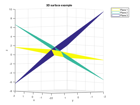
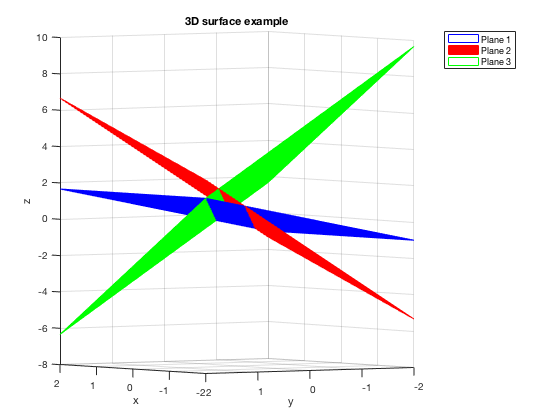
Changing Colors of Surfaces, Example 1

There are several ways to do this, many of them get really fancy. Here's one basic example.

xd=linspace(-2,2,40);
yd=linspace(-2,2,40);
[x,y]=meshgrid(xd,yd);
% first plane
a1=0;
b1=-2;
c1=3;
d1=1;
z1=-a1/c1*x-b1/c1*y+d1/c1;
% second plane
a2=3;
b2=6;
c2=-3;
d2=-2;
z2=-a2/c2*x-b2/c2*y+d2/c2;
% third plane
a3=6;
b3=6;
c3=3;
d3=5;
z3=-a3/c3*x-b3/c3*y+d3/c3;
mesh(x,y,z1,'EdgeColor','blue')
hold on
surf(x,y,z2,'EdgeColor','red', 'FaceColor', 'red')
mesh(x,y,z3,'EdgeColor', 'green')
title('3D surface example')
xlabel('x'), ylabel('y'), zlabel('z')
legend('Plane 1', 'Plane 2', 'Plane 3')
view(-125,2)
hold off

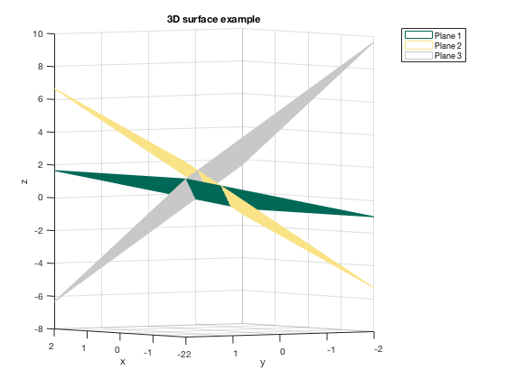
Changing Colors of Surfaces, Example 2

Here's another way, using RGB codes for colors:

xd=linspace(-2,2,40);
yd=linspace(-2,2,40);
[x,y]=meshgrid(xd,yd);
C1=(1/255)*[0,104,87];     % establishing color of first plane: Loyola Green
C2=(1/255)*[250,227,135];  % establishing color of second plane: Loyola Gold
C3=(1/255)*[200,200,200];  % establishing color of third plane: Loyla Gray
% first plane
a1=0;
b1=-2;
c1=3;
d1=1;
z1=-a1/c1*x-b1/c1*y+d1/c1;
% second plane
a2=3;
b2=6;
c2=-3;
d2=-2;
z2=-a2/c2*x-b2/c2*y+d2/c2;
% third plane
a3=6;
b3=6;
c3=3;
d3=5;
z3=-a3/c3*x-b3/c3*y+d3/c3;
mesh(x,y,z1,'EdgeColor',C1)
hold on
mesh(x,y,z2,'EdgeColor',C2)
mesh(x,y,z3,'EdgeColor',C3)
title('3D surface example')
xlabel('x'), ylabel('y'), zlabel('z')
legend('Plane 1', 'Plane 2', 'Plane 3')
view(-125,2)
hold off

Changing Colors of Surfaces, Example 3

Here's another way.

xd=linspace(-2,2,40);
yd=linspace(-2,2,40);
[x,y]=meshgrid(xd,yd);
C1=0*x+100;     % color of first plane
C2=0*x;         % color of second plane
C3=0*x-100;     % color of third plane
% first plane
a1=0;
b1=-2;
c1=3;
d1=1;
z1=-a1/c1*x-b1/c1*y+d1/c1;
% second plane
a2=3;
b2=6;
c2=-3;
d2=-2;
z2=-a2/c2*x-b2/c2*y+d2/c2;
% third plane
a3=6;
b3=6;
c3=3;
d3=5;
z3=-a3/c3*x-b3/c3*y+d3/c3;
mesh(x,y,z1,C1)
hold on
mesh(x,y,z2,C2)
mesh(x,y,z3,C3)
title('3D surface example')
xlabel('x'), ylabel('y'), zlabel('z')
legend('Plane 1', 'Plane 2', 'Plane 3')
view(-125,2)
hold off

M-file that created this page

BACK TO MAIN PLOTTING PAGE

Published with MATLAB® R2016a