Different Coordinate Systems
L. Oberbroeckling, Fall 2011.
This has a lot of stuff; read the contents carefully!
NOTE: m-files don't view well in Internet Explorer. Use Mozilla Firefox or Safari instead to view these pages.
Contents
You may want to have the following commands at the top of your script files to "start fresh"
clc         % clears the command window
clear       % clears ALL variables
format      % resets the format to the default format
There are many other examples on the H-drive!
There are several ways to produce graphs of functions. This page will not show all of them; it will show the way that is the most customizable and can be easily extended to more complicated settings (like parametric equations, 3D, etc.) This is also a learn-by-example page. I do not explain every command or show everything. It is up to you to experiment and look up these commands to better understand them.
To plot in a different coordinate system, the commands sph2cart and pol2cart come in handy. First set up your domains and formulas within that coordinate system as you normally would. Use the commands mentioned above and below to create your variables x, y or x,y,z. Then use plot(x,y), mesh(x,y,z), etc. as you normally would along with the typical formatting commands.
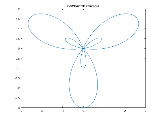
Polar Coordinates
If in polar, you'd use [x,y]=pol2cart(theta, r);. (Or you could do it brute-force!)
t=linspace(0,2*pi,300);     % as always, you have to be careful so graph isn't jagged, etc.
r=1+2*sin(3*t);
[x,y]=pol2cart(t,r);
plot(x,y)
title('Pol2Cart 2D Example')
Or you could do the conversions brute-force.
t=linspace(0,2*pi,300);     % as always, you have to be careful so graph isn't jagged, etc.
r=1+2*sin(3*t);
x=r.*cos(t); y=r.*sin(t);
plot(x,y)
title('Pol2Cart 2D Example')

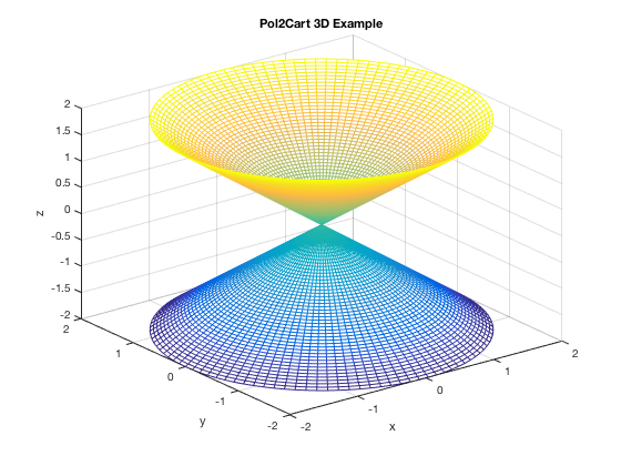
Cylindrical Coordinates
If using Cylindrical coordinates, you still use the same command as above, except that you'd have [x,y,z]=pol2cart(theta, r, z); (or convert brute-force).
t=linspace(0,2*pi); % as always, you have to be careful so graph isn't jagged, etc.
r=linspace(-2,2);
[t,r]=meshgrid(t,r);
z=r;
[x,y,z]=pol2cart(t,r,z);
mesh(x,y,z)
xlabel('x')
ylabel('y')
zlabel('z')
title('Pol2Cart 3D Example')
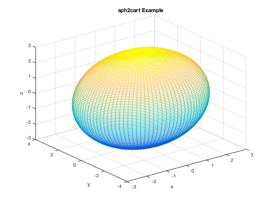
Spherical Coordinates
Use [x,y,z]=sph2cart(theta, phi, rho);. NOTE: phi is defined differently in MATLAB than in our book! (see MATLAB help). The book has phi defined as the angle of rotation from the positive z-axis, while MATLAB defines it as the angle of elevation from the xy-plane. According to the book's definition of phi, phi = 0 would be pointing straight upwards, phi = pi/2 would be exactly horizontal and phi = pi pointing straight downwards. According to MATLAB's definition, phi = pi/2 would be pointing exactly straight upwards, phi = 0 would be exactly horizontal and phi = -pi/2 pointing straight downwards.
theta=linspace(0,2*pi); % as always, you have to be careful so graph isn't jagged, etc.
phi=linspace(-pi/2,pi/2);
[t,p]=meshgrid(theta, phi);
rho = 3+0*t;
[x,y,z]=sph2cart(t,p,rho);
mesh(x,y,z)
title('sph2cart Example')
xlabel('x'), ylabel('y'), zlabel('z')
Mixing Coordinate systems 2D
You just add plot commands using HOLD ON/HOLD OFF
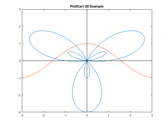
t=linspace(0,2*pi);     % as always, you have to be careful so graph isn't jagged, etc.
r=1+2*sin(3*t);
[x,y]=pol2cart(t,r);
plot(x,y)
title('Pol2Cart 2D Example')
hold on
x2=linspace(-3,3);
y2 = cos(x2);
plot(x2,y2)
yh = 0*x2;
yv = linspace(-3,3);
xv = 0*yv;
plot(x2,yh,'k',xv,yv,'k')
hold off
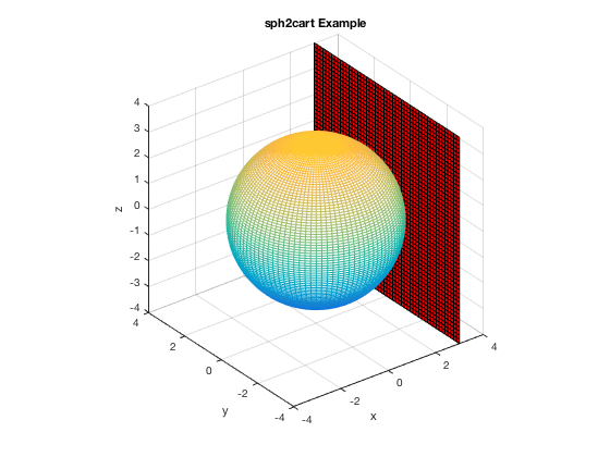
Mixing Coordinate Systems 3D, Vertical Plane Example
As in the 2D case, you just use HOLD ON/HOLD OFF
clear
theta=linspace(0,2*pi); % as always, you have to be careful so graph isn't jagged, etc.
phi=linspace(-pi/2,pi/2);
[t,p]=meshgrid(theta, phi);
rho = 3+0*t;
[x,y,z]=sph2cart(t,p,rho);
mesh(x,y,z)
title('sph2cart Example')
xlabel('x'), ylabel('y'), zlabel('z')
% vertical plane set-up and plot
yd=linspace(-4,4,51);
zd=linspace(-4,4,51);
[y2,z2]=meshgrid(yd,zd);
x2=3 + 0*z2;
hold on
surf(x2,y2,z2,'FaceColor', 'red')
axis square
hold off