Parametric Equations, Vector Functions, and Fine-Tuning Plots

L. Oberbroeckling, updated January 2018.

NOTE: m-files don't view well in Internet Explorer. Use Mozilla Firefox or Safari instead to view these pages.

2D Parametric Equations
Bad Domain Example
Better Domain
3D Parametric Equation (Vector Equation) Example
Multiple Graphs Using HOLD ON
Getting a Different 3D View
Plotting Points
Thicker Lines
Plotting a Point
Making the Point Bigger (and different)
Fine-tuning the Ranges of the Axes
Creating a Legend
M-file that created this page
BACK TO MAIN PLOTTING PAGE

You may want to have the following commands at the top of your script files to "start fresh"

clc         % clears the command window
clear       % clears ALL variables
format      % resets the format to the default format

Loyola Peeps: There are many other examples on the H-drive!

There are several ways to produce graphs of functions. This page will not show all of them; it will show the way that is the most customizable and can be easily extended to more complicated settings (like parametric equations, 3D, etc.) This is also a learn-by-example page. I do not explain every command or show everything. It is up to you to experiment and look up these commands to better understand them.

To plot vector functions or parametric equations, you follow the same idea as in plotting 2D functions, setting up your domain for t. Then you establish x, y (and z if applicable) according to the equations, then plot using the plot(x,y) for 2D or the plot3(x,y,z) for 3D command.

2D Parametric Equations

Here are some parametric equations that you may have seen in your calculus text (Stewart, Chapter 10).

\[x = 1.5\cos t - \cos(10t)\] \[y = 1.5\sin t - \sin(10t)\]

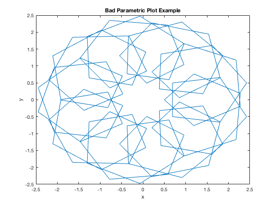
Bad Domain Example

t=linspace(0,4*pi);
x = 1.5*cos(t) - cos(10*t);
y = 1.5*sin(t) - sin(10*t);
plot(x,y);
xlabel('x'),ylabel('y')
title('Bad Parametric Plot Example')

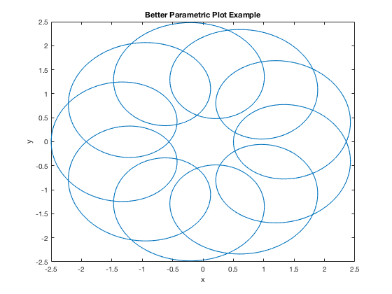
Better Domain

Notice the plot above is extremely jagged. That is because our domain is too "rough" - there aren't enough points plotted. This is a case where we want to increase number of elements in our x vector.

t=linspace(0,4*pi, 1000);
x = 1.5*cos(t) - cos(10*t);
y = 1.5*sin(t) - sin(10*t);
plot(x,y);
xlabel('x'),ylabel('y')
title('Better Parametric Plot Example')

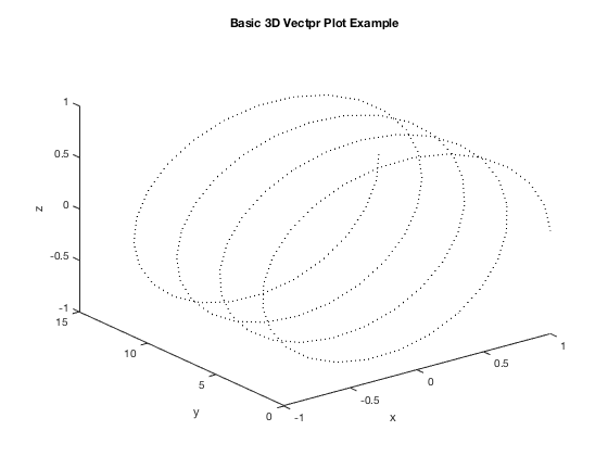
3D Parametric Equation (Vector Equation) Example

t=linspace(0,4*pi);
x = cos(2*t);
y = t;
z = sin(2*t);
plot3(x,y,z, 'k:'); % the 'k:' command makes the line black and dotted

xlabel('x'),ylabel('y'),zlabel('z')
title('Basic 3D Vectpr Plot Example')

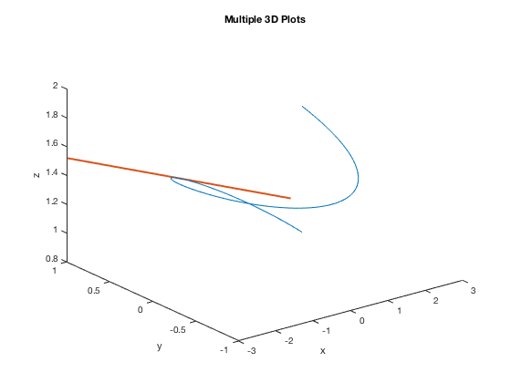
Multiple Graphs Using HOLD ON

This example shows how to plot more than one on the same graph and how to change some features of the graph

t = linspace(0,2*pi);
x=cos(t);
y=sin(t);
z=exp(t/10);
plot3(x,y,z)
xlabel('x'),ylabel('y'),zlabel('z')
% setting up second plot
hold on  % command needed to put more plots on same figure
s=linspace(-3,3);
x2=-s;
y2=1+0*s;
z2=exp(pi/20) + 1/10*exp(pi/20)*s;
plot3(x2,y2,z2,'LineWidth',2)
title('Multiple 3D Plots')
hold off  % command needed when done with all plots for figure

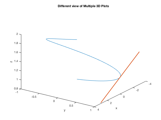
Getting a Different 3D View

This is the same graph as the one above, but getting a different view using view command in order to see that the line segment is tangent to the curve. This example shows how to plot more than one on the same graph and how to change some features of the graph. This command may take some reading, some practice and even a few runs with different settings to get the correct view.

t = linspace(0,2*pi);
x=cos(t);
y=sin(t);
z=exp(t/10);
plot3(x,y,z)
xlabel('x'),ylabel('y'),zlabel('z')
% setting up second plot
hold on
s=linspace(-3,3);
x2=-s;
y2=1+0*s;
z2=exp(pi/20) + 1/10*exp(pi/20)*s;
plot3(x2,y2,z2,'LineWidth',2)
title('Different view of Multiple 3D Plots')
view(125,30)        % changes perspective - experiment with these numbers
hold off

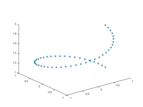
Plotting Points

Many of the following work for both the 2D and 3D figures. If we wanted just a plot of points rather than connecting them with a line, we specify a "marker style". Common ones are ., d, *, o.

t = linspace(0,2*pi, 50);
x=cos(t);
y=sin(t);
z=exp(t/10);
plot3(x,y,z, '*')

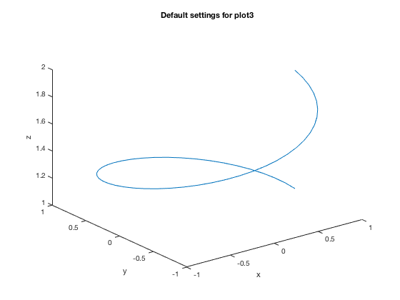
Thicker Lines

Original, default plot

plot3(x,y,z)
xlabel('x'),ylabel('y'),zlabel('z')
title('Default settings for plot3')

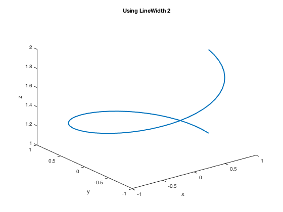
Using the following LineWidth setting changes the thickness of the line. The default width is 0.5 points.

plot3(x,y,z,'LineWidth',2)
xlabel('x'),ylabel('y'),zlabel('z')
title('Using LineWidth 2')

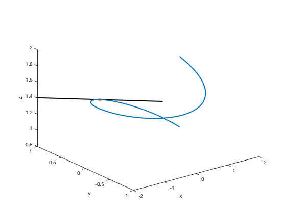
Plotting a Point

Similarly done as in the 2D case

plot3(x,y,z,'LineWidth',2)
xlabel('x'),ylabel('y'),zlabel('z')
hold on  % command needed to put more plots on same figure
s=linspace(-2,2);
x2=-s;
y2=1+0*s;
z2=exp(pi/20) + 1/10*exp(pi/20)*s;
plot3(x2,y2,z2,'k','LineWidth',2)
plot3(0, 1, exp(pi/20), 'o') % marks the point with a green "o"
hold off

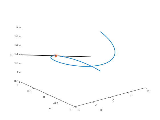
Making the Point Bigger (and different)

Notice that you can barely see the point in the graph above. You may want to change the color, shape, and/or size to make it stand out more and you may need to experiment with different settings. Here we're making the point be a "*" and make it bigger using the MarkerSize setting. Default value for MarkerSize is 6.

plot3(x,y,z,'LineWidth',2)
xlabel('x'),ylabel('y'),zlabel('z')
hold on  % command needed to put more plots on same figure
s=linspace(-2,2);
x2=-s;
y2=1+0*s;
z2=exp(pi/20) + 1/10*exp(pi/20)*s;
plot3(x2,y2,z2,'k','LineWidth',2)
plot3(0, 1, exp(pi/20), '*', 'MarkerSize', 10)
hold off

You can also change the way the marker looks by also specifying a different LineSize (default is 0.5 points).

plot3(x,y,z,'LineWidth',2)
xlabel('x'),ylabel('y'),zlabel('z')
hold on  % command needed to put more plots on same figure
s=linspace(-2,2);
x2=-s;
y2=1+0*s;
z2=exp(pi/20) + 1/10*exp(pi/20)*s;
plot3(x2,y2,z2,'k','LineWidth',2)
plot3(0, 1, exp(pi/20), '*', 'MarkerSize', 10, 'LineWidth', 2)
hold off

There are other settings you can adjust, like MarkerEdgeColor, MarkerFaceColor, etc. For more information (probably more than you want to know), go to MathWorks documentation

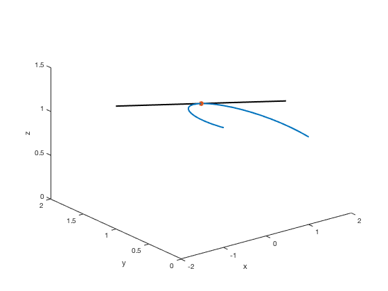
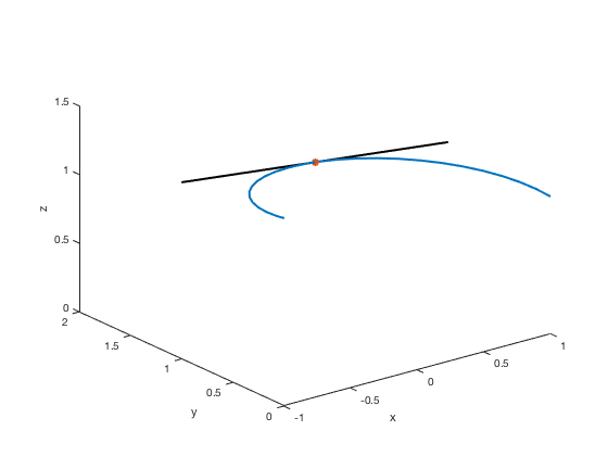
Fine-tuning the Ranges of the Axes

plot3(x,y,z,'LineWidth',2)
xlabel('x'),ylabel('y'),zlabel('z')
hold on  % command needed to put more plots on same figure
s=linspace(-2,2);
x2=-s;
y2=1+0*s;
z2=exp(pi/20) + 1/10*exp(pi/20)*s;
plot3(x2,y2,z2,'k','LineWidth',2)
plot3(0, 1, exp(pi/20), '*', 'LineWidth', 2)
hold off
ylim([0,2])
zlim([0,1.5])
hold off

Another way is to use the axis command to set all limits at once with the order xmin, xmax, ymin, ymax, zmin, zmax.

plot3(x,y,z,'LineWidth',2)
xlabel('x'),ylabel('y'),zlabel('z')
hold on  % command needed to put more plots on same figure
s=linspace(-2,2);
x2=-s;
y2=1+0*s;
z2=exp(pi/20) + 1/10*exp(pi/20)*s;
plot3(x2,y2,z2,'k','LineWidth',2)
plot3(0, 1, exp(pi/20), '*', 'LineWidth', 2)
hold off
axis([-1, 1, 0, 2, 0, 1.5])
hold off

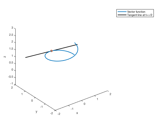
Creating a Legend

plot3(x,y,z,'LineWidth',2)
xlabel('x'),ylabel('y'),zlabel('z')
hold on  % command needed to put more plots on same figure
s=linspace(-2,2);
x2=-s;
y2=1+0*s;
z2=exp(pi/20) + 1/10*exp(pi/20)*s;
plot3(x2,y2,z2,'k','LineWidth',2)
plot3(0, 1, exp(pi/20), 'o', 'LineWidth', 2)
hold off
axis([-2, 2, -2, 2, -1, 3])
legend('Vector function', 'Tangent line at t=\pi/2')