Colors in MATLAB plots

L. Oberbroeckling, Spring 2018.

Default Colors in 2D Graphs
Default Colors in 3D Graphs
Using Basic Colors in Graphs
Changing Colors
Using RGB triplets to change colors
Changing colors in 3D Graphs
m-file that created this page
BACK TO MAIN PLOTTING PAGE

This document gives BASIC ways to color graphs in MATLAB. See

http://www.mathworks.com/help/matlab/visualize/coloring-mesh-and-surface-plots.html

and

http://www.mathworks.com/help/matlab/ref/colormap.html

for more in-depth explanations and fancier coloring, to name just two sources.

Default Colors in 2D Graphs

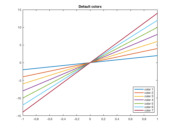
The default colors used in MATLAB changed in R2014b version. Here are the colors, in order, and their MATLAB RGB triplet.

Current color Old color

           [0, 0.4470, 0.7410]            [0, 0, 1]

           [0.8500, 0.3250, 0.0980]            [0, 0.5, 0]

           [0.9290, 0.6940, 0.1250]            [1, 0, 0]

           [0.4940, 0.1840, 0.5560]            [0, 0.75, 0.75]

           [0.4660, 0.6740, 0.1880]            [0.75, 0, 0.75]

           [0.3010, 0.7450, 0.9330]            [0.75, 0.75, 0]

           [0.6350, 0.0780, 0.1840]            [0.25, 0.25, 0.25]

Current color	Old color
	[0, 0.4470, 0.7410]		[0, 0, 1]
	[0.8500, 0.3250, 0.0980]		[0, 0.5, 0]
	[0.9290, 0.6940, 0.1250]		[1, 0, 0]
	[0.4940, 0.1840, 0.5560]		[0, 0.75, 0.75]
	[0.4660, 0.6740, 0.1880]		[0.75, 0, 0.75]
	[0.3010, 0.7450, 0.9330]		[0.75, 0.75, 0]
	[0.6350, 0.0780, 0.1840]		[0.25, 0.25, 0.25]

x=linspace(-1,1);
plot(x,2*x, x,4*x, x,6*x, x,8*x, x,10*x, x,12*x, x,14*x, 'LineWidth', 2)
legend('color 1', 'color 2', 'color 3', 'color 4', 'color 5', 'color 6', 'color 7', 'Location', 'SouthEast')
title('Default colors')

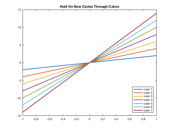
Another thing that changed starting in the R2014b version is that the hold on and hold off automatically cycles through the colors. In the past, each new plot command would start with the first color (blue) and you would have to manually change the color. Now it will automatically move to the next color(s). See below for how to manually adjust the colors.

plot(x,2*x, 'LineWidth', 2)
hold on
plot(x,4*x, 'LineWidth', 2)
plot(x,6*x, 'LineWidth', 2)
plot(x,8*x, 'LineWidth', 2)
plot(x,10*x, 'LineWidth', 2)
plot(x,12*x, 'LineWidth', 2)
plot(x,14*x, 'LineWidth', 2)
hold off
legend('color 1', 'color 2', 'color 3', 'color 4', 'color 5', 'color 6', 'color 7', 'Location', 'SouthEast')
title('Hold On Now Cycles Through Colors')

Default Colors in 3D Graphs

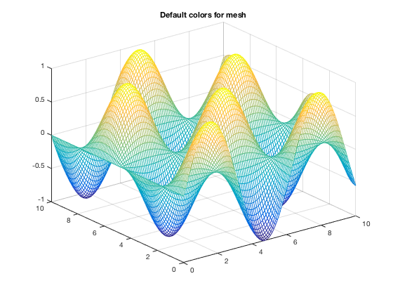
If using mesh(x,y,z), to change the look of it you would want to change 'EdgeColor'. Note that the name of this colormap is "parula" while previous to R2014b, it was "jet"

[x,y]=meshgrid(linspace(0,10));
z=sin(x).*cos(y);
mesh(x,y,z)
title('Default colors for mesh')

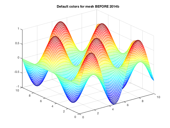
[x,y]=meshgrid(linspace(0,10));
z=sin(x).*cos(y);
mesh(x,y,z)
colormap(jet)
title('Default colors for mesh BEFORE 2014b')

Using Basic Colors in Graphs

The eight basic colors are known by either their short name or long name (RGB triplets are also included).

Long Name Short Name RGB Triplet

blue b [0,0,1]

black k [0,0,0]

red r [1,0,0]

green g [0,1,0]

yellow y [1,1,0]

cyan c [0,1,1]

magenta m [1,0,1]

white w [1,1,1]

Long Name	Short Name	RGB Triplet
blue	b	[0,0,1]
black	k	[0,0,0]
red	r	[1,0,0]
green	g	[0,1,0]
yellow	y	[1,1,0]
cyan	c	[0,1,1]
magenta	m	[1,0,1]
white	w	[1,1,1]

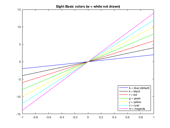
Example of how to change the color using short names is below. You can easily do the same thing using the long names.

x=linspace(-1,1);
plot(x,2*x,'b')
hold on
plot(x,4*x,'k')
plot(x,6*x,'r')
plot(x,8*x,'g')
plot(x,10*x,'y')
plot(x,12*x,'c')
plot(x,14*x,'m')
hold off
legend('b = blue (default)', 'k = black', 'r = red', 'g = green', 'y = yellow', 'c = cyan', 'm = magenta', 'Location', 'SouthEast')
title('Eight Basic colors (w = white not drawn)')

Changing Colors

Many times you want to have more control of what colors are used. For example, I may want some data points drawn in the same color as the curve. Or I have a piece-wise graph that I want to have all the same color. There are several ways to do this. One is to use the default colors and "resetting" the order, which is shown here. Others involve using the RGB triplet (see next section).

x=linspace(-10,10); y=3*sin(x);
xp=[0:pi/2:10]; yp=3*sin(xp);
x1 = linspace(-10,-0.1); x2=linspace(0.1,10);
y1=1./x1; y2=1./x2;
plot(x,y)
hold on
ax = gca;
ax.ColorOrderIndex = 1;
plot(xp,yp,'*')
plot(x1,y1)
ax.ColorOrderIndex = 2;
plot(x2,y2)
hold off
axis equal

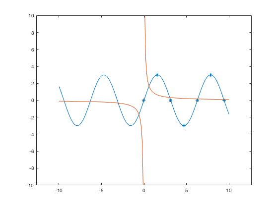
As you may see, this could get confusing to keep track of. Thus it may be easier to use the RGB triplets, and even name them ahead of time. This is discussed in the section below.

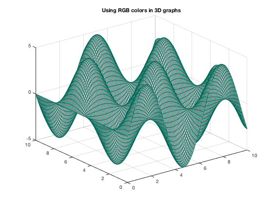
Using RGB triplets to change colors

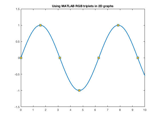
One can specify colors using a vector that gives the RGB triple where in MATLAB, each of the three values are numbers from 0 to 1. Usually RGB colors have values from 0 to 255. You can use those numbers and divide the vector by 255 to use within MATLAB. Thus knowing the MATLAB RGB triples for the colors can be useful. From the table above, we can define the default colors to work with them or can put in the RGB triplet (as a vector) directly into the plot command. Both are shown in this example.

color1=[0,0.4470, 0.7410];
t=linspace(0,10);
t2=0:pi/2:10;
plot(t,sin(t), 'LineWidth',2)
hold on
plot(t2,sin(t2),'s','MarkerEdge',color1,'MarkerFace',[0.9290,0.6940, 0.1250],'MarkerSize',9)
hold off
ylim([-1.5,1.5])
title('Using MATLAB RGB triplets in 2D graphs')

For other colors, you can look up their RGB code on many websites such as RGB Color Codes Chart or HTML Color Picker to see the RGB codes (or hex codes, etc.) For example, at these RGB Color websites, you will be given R=255, G=0, B=0 for red. So you can use 1/255[255,0,0] to get the color of red to use as a color in MATLAB.

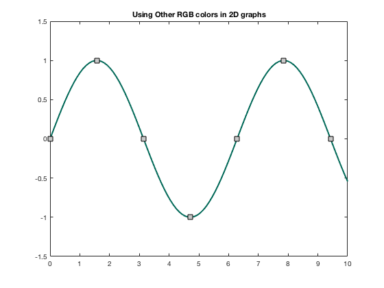
The official color for Loyola Green is given as RGB:0-104-87, and Loyola Gray is given as RGB:200-200-200 (found on Loyola's Logos/University Signature page. Here's how one can use those colors in MATLAB.

loyolagreen = 1/255*[0,104,87];
loyolagray = 1/255*[200,200,200];

Now one can use these colors to specify the color of markers, lines, edges, faces, etc.

t=linspace(0,10);
t2=0:pi/2:10;
plot(t,sin(t),'Color', loyolagreen, 'LineWidth',2)
hold on
plot(t2,sin(t2),'s','MarkerEdge','k','MarkerFace',loyolagray,'MarkerSize',9)
hold off
ylim([-1.5,1.5])
title('Using Other RGB colors in 2D graphs')

Changing colors in 3D Graphs

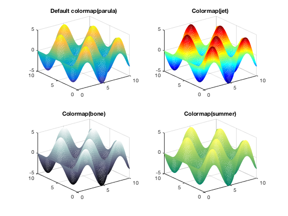
If using mesh(x,y,z), to change the look of it you can change to a different colormap as discussed in https://www.mathworks.com/help/matlab/ref/colormap.html. This was done above when showing the previous default colormap. Here are some more.

Warning! Once you change the colormap, it will keep that colormap for all subsequent 3D plots within the same figure or MATLAB session until you use close, or open a new figure window.

[x,y]=meshgrid(linspace(0,10));
z=5*sin(x).*cos(y);
ax1=subplot(2,2,1);
    mesh(x,y,z)
    colormap(ax1,parula)
    title('Default colormap(parula)')
ax2=subplot(2,2,2);
    mesh(x,y,z)
    colormap(ax2,jet)
    title('Colormap(jet)')
ax3=subplot(2,2,3);
    colormap(ax3,bone)
    mesh(x,y,z)
    title('Colormap(bone)')
ax4=subplot(2,2,4);
    colormap(ax4,summer)
    mesh(x,y,z)
    title('Colormap(summer)')

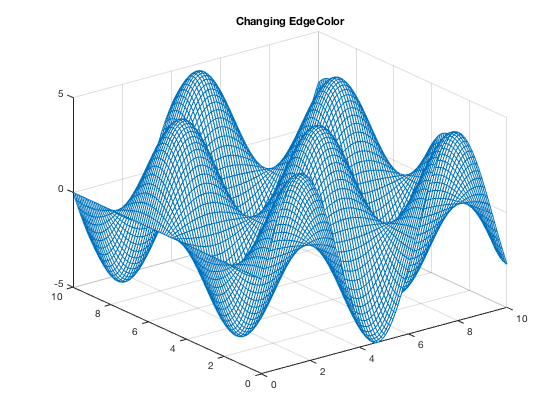
For mesh and surf, you can change 'EdgeColor' and/or 'FaceColor' to be uniform, rather than using colormaps.

close all           %  to reset the colormap
mesh(x,y,z,'EdgeColor',color1)
title('Changing EdgeColor')

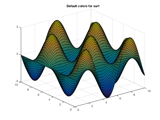
Note that you can get as fancy as you want with your own coloring
schemes.  These are discussed in MATLAB's documentation (and elsewhere!)
but I am not discussing here.

surf(x,y,z)
title('Default colors for surf')

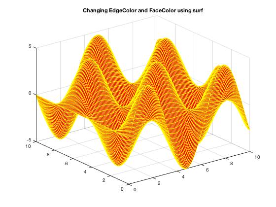
surf(x,y,z,'EdgeColor', 'y', 'FaceColor','r')
title('Changing EdgeColor and FaceColor using surf')

surf(x,y,z,'EdgeColor',loyolagreen,'FaceColor',loyolagray)
title('Using RGB colors in 3D graphs')