|
For this week's assignment, we are interested in playing with photographs. To be able to import photos into Matlab, we can use the following commands:
>>img = imread('photo.jpg');
However, this imports the image as an array of uint8 data as the sample size for each color component is 8 bits. In order for us to 'play' with this data, we have to convert it to double data. This can easily be done by typing
>>img = im2double(img);
Now we can ask Matlab to show the image by typing
>>imshow(img)
If you input a color image, Matlab stores this as a three-dimensional array, as it uses RGB values. Thus,
img(:,:,1) represents the Red values
img(:,:,2) represents the Green values
img(:,:,3) represents the Blue values
To gain intuition, type the following into Matlab
>> Z = zeros(20,60,3);
>> Z(:,:,1) = [ones(20,20) zeros(20,20) zeros(20,20)];
>> Z(:,:,2) = [zeros(20,20) ones(20,20) zeros(20,20)];
>> Z(:,:,3) = [zeros(20,20) zeros(20,20) ones(20,20)];
>> imshow(Z)
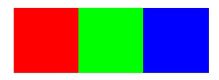
Note that the first 20x20 pixels are red, the second 20x20 pixels are green, and the last 20x20 pixels blue. Can you understand why?
Now type the following into Matlab
>> Z(:,:,2) = [zeros(20,20) ones(20,20) ones(20,20)];
>> imshow(Z)
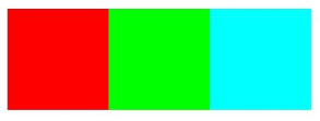
Notice the difference. The last square has turned cyan. Note, that many times the range values for RBG are between 0 and 255 such as in here. Can you figure out how to scale them so that they are from 0 and 1? Experiment with different values in the squares. Note that for simplicity the numbers should be between 0 and 1.
You should now understand that color photographs are just be a bunch of pixels composed of RGB values. And, that these pixel values can be stored in 3-dimensional arrays. As a result, we can start manipulating images in Matlab using matrix manipulations as will be shown with the following problem set.
Convolutions
One of the most common manipulations with images deals with convolutions. This operation is able to bring out certain features in an image. Typically, convolutions are defined on functions f and g as
\[(f*g)(t) = \int_\infty^\infty f(t-\tau)g(\tau)d\tau\]
However, this operation can be discritized so that it is defined as
\[(f*g)[n] = \sum_{m=-\infty}^\infty f[n-m]g[m]\]
For images, a further simplification can be done. We can think of f as a function that relates the pixel location to an RGB value and g as a kernel that acts on the image. For example, imagine that the red values of a color image are the following
\[\begin{array}{c c c c}
1& 1/2 & 1/3 & 1/4\\
1& 1/3 & 1/4 & 1/5\\
1& 1/2 & 1/2 & 1/2
\end{array}\]
and assume that the kernel is
\[\begin{array}{ccc}
1 & 2 & 1\\1 & 1 & 1\\1 & 2 & 1
\end{array}\]
We can apply this kernel to the image twice as the 3x3 kernel can only fit the 3x4 matrix in two positions. In the first position, we can element wise multiply the kernel with the left 3x3 block of the image and sum the values.
\[1*1 + 1/2*2 + 1/3*1 + 1*1 + 1/3*1 + 1/4*1 + 1*1 + 1/2*2 + 1/2*1 = 77/12\]
Note that this value is above 1. To fix this, the kernel should be normalized. To do this, we divide each element in the kernel by the sum of all the absolute values of the elements in the kernel. Normalization ensures that the pixel values in the output image are of the same relative magnitude as those in the input image.
So our kernel would now be
\[\begin{array}{ccc}
1/11 & 2/11 & 1/11\\1/11 & 1/11 & 1/11\\1/11 & 2/11 & 1/11
\end{array}\]
which would result in the convolution to be 7/12. Similary the second position would give you 21/55. As a result our new image would have red values of
\[\begin{array}{c c c c}
1& 1/2 & 1/3 & 1/4\\
1& 7/12 & 21/55 & 1/5\\
1& 1/2 & 1/2 & 1/2
\end{array}\]
You could do this for each color matrix in your three dimensional array, scrolling across the image. In the problem set, you will build your own convolution operator.
Problem Set 4
- Create an m-file called hw4Last.m where Last is the first four letters of your last name in your MA302 folder. You should now have the tools to create your own published files by adapting your previous homework. Note that I will be grading format starting this week. Your published file should be polished as if you were to turn it in as a final report.
- Import your favorite jpeg into Matlab and store it in a matrix img. Switch the Blue and Green values and store the image in a matrix new. Comment on how this effects your image. Next, play with tolerances to enhance certain color regions in your photo. Once you are happy with the image, store it in a matrix enhanced. Comment on why you are happy with the final image. Display the original image img, the blue and green switched image new, and the enhanced image enhanced in one figure. Hint: Google is your friend.
Note that you should experiment in the command window before publishing your commands in hw4Last.m I should just be able to copy paste your code to see your results. Any mistakes/experimentation should not be included in your published file.
- Write a script convLast.m that applies a convolution to img with the kernel K defined outside your script. First, apply the kernel
\[\begin{array}{ccc}
1&1&1\\
1&1&1\\
1&1&1
\end{array}\]
to img to create kerLast1. Don't forget to normalize the kernel! What effect does this kernel have on your image? Does it make sense why?
Next, apply the kernel
\[\begin{array}{ccc}
0&-1&0\\
-1&4&-1\\
0&-1&0
\end{array}\]
to img to create kerLast2 Don't forget to normalize the kernel! What effect does this kernel have on your image?
Now create your own kernel and apply it to img to create kerLast3. Display img, kerLast1, kerLast2, kerLast3 in one figure.
With this problem do not forget that the convolutions must be applied to ALL THREE RBG values!
- Post your m-file hw4Last.m to dropittome using the same password as we used in the first homework. In order to get full credit, your directories and files must be named correctly and you must have links to your function file and the m-file (script file) that created the webpage, along with the appropriate text, plots, and such to answer the problems.
|