|
For this week's assignment, we will be learning how to import data and analyze it with Matlab. Data can be stored in a variety of formats from csv files to excel files. For this assignment we will work with csv files. You can load data into Matlab using the comand importdata. Download the Data into your current directory. This data gives the preference of 100 people to 60 different types of movies. The data was collected by Dr. Rick Auer for his ST472 class. If you enjoy this assignment, you may want to consider taking Applied Multivariate Analysis.
Now to load the data type the following command
>>A = importdata('movData.csv',',',1);
Type help importdata to understand what the inputs represent. You now have an array of data. To access the first header elements you would type
>>disp(A.colheaders{1,1})
which returns personal relationships which is the first movie genre in the csv file. Now to access the actual data, we will create a matrix M that contains the numeric values by typing
>>M = A.data(:,:);
Now all of the numeric data in the csv file is stored in the variable M. We can now run a bunch of mathematics on the data to analyze it -- FUN! For example, we can see which genre has the highest ranking by typing
>> [m,in]=max(sum(M));
>> disp(A.colheaders{1,in})
A very typical question that may come up is how does one theme relate to another. In order to create such an understanding we can use MATHEMATICS!
Covariance Matrix
Here we will study the covariance matrix. In order to understand the covariance matrix, it is useful to first understand the variance of an element. The variance describes how spread out are a set of numbers $\{x_i\}$. Mathematically, this is represented as
\[s^2 = \frac{1}{n}\sum_{i=1}^n (x_i-\mu)^2=\frac{1}{n}\sum_{i=1}^n (x_i-\mu)(x_i-\mu)\]
where $n$ is the number of elements in the set and $\mu$ is the mean of the $x_i$. Note the notation for variance is $s^2$ which is the square of the standard deviation represented as $s$. Similarly, we can describe how two vectors $\mathbf{x}=[x_1,x_2,\ldots,x_n]^T$ and $\mathbf{y}=[y_1,y_2,\ldots,y_n]^T$ vary (co-vary) by looking at the covariance
\[cov(\mathbf{x},\mathbf{y})=\frac{1}{n}\overline{\mathbf{x}}^T\overline{\mathbf{y}}=\frac{1}{n}\sum_{i=1}^n (x_i-\mu_x)(y_i-\mu_y)\]
Here $\overline{\mathbf{x}}$ stands for the mean-centered $\mathbf{x}$. Now let's see if this makes sense. Note that the inner product defines the $\cos\theta$ between the two vectors. Therefore, if the two vectors are close together $\theta\approx 0$ and $\cos\theta \approx 1$. Similarly, if two vectors are spread apart then $\theta\approx\pi/2$ and $\cos\theta\approx 0$. As a result, if two vectors $\mathbf{x}$ and $\mathbf{y}$ are close together then $cov(\mathbf{x},\mathbf{y})$ will be large.
In our example, we have data that are represented in a matrix. Each column represents a different variable. Therefore, if we take the covariance of each column we will know how each columns covaries with another. We can represent this with a covariance matrix:
\[
\mathbf{CovMat} =
\begin{pmatrix}
cov(\mathbf{x}_1,\mathbf{x}_1) & cov(\mathbf{x}_1,\mathbf{x}_2) &\cdots&cov(\mathbf{x}_1,\mathbf{x}_n)\\
cov(\mathbf{x}_2,\mathbf{x}_1) & cov(\mathbf{x}_2,\mathbf{x}_2) &\cdots&cov(\mathbf{x}_2,\mathbf{x}_n)\\
\vdots&\vdots&\ddots&\vdots\\
cov(\mathbf{x}_n,\mathbf{x}_1) & cov(\mathbf{x}_n,\mathbf{x}_2) &\cdots&cov(\mathbf{x}_n,\mathbf{x}_n)\\
\end{pmatrix}
\]
Note that each term is divided by $n$. There are statistical reasons for dividing by $n-1$ instead of $n$. However, to keep things simple we will use $n$.
Correlation Matrix
The way that we have defined the covariance matrix, it is hard to tell how one column of the covariance matrix relates to another. To make the results easier to compare, one often divides the $(i,j)$th entry of $\mathbf{C}$ by $\sigma_i\sigma_j$ where the standard deviation of $\mathbf{x}_i$ is represented by $\sigma_i$. This is known as a correlation matrix. The resulting matrix is symmetric with $1$s on the diagonal.
\[
\mathbf{CorMat} =
\begin{pmatrix}
1 & \frac{cov(\mathbf{x}_1,\mathbf{x}_2)}{\sigma_1\sigma_2} &\cdots&\frac{cov(\mathbf{x}_1,\mathbf{x}_n)}{\sigma_1\sigma_n}\\
\frac{cov(\mathbf{x}_2,\mathbf{x}_1)}{\sigma_2\sigma_1} & 1&\cdots&\frac{cov(\mathbf{x}_2,\mathbf{x}_n)}{\sigma_2\sigma_n}\\
\vdots&\vdots&\ddots&\vdots\\
\frac{cov(\mathbf{x}_n,\mathbf{x}_1)}{\sigma_n\sigma_1} & \frac{cov(\mathbf{x}_n,\mathbf{x}_2)}{\sigma_n\sigma_2} &\cdots&1\\
\end{pmatrix}
\]
Principal Component Analysis
When you have a lot of data you may want to know which variables are highly correlated with one another. You can do this with a method known as Principal Component Analysis (PCA). The idea works by trying to find a vector $\mathbf{x}$ such that
\[\frac{\mathbf{x}^T\mathbf{A}^T\mathbf{A}\mathbf{x}}{\mathbf{x}^T\mathbf{x}}\]
is as large as possible for the data stored in a matrix $\mathbf{A}$. Let's assume that $\mathbf{A}$ is mean centered, then $\mathbf{A}^T\mathbf{A}$ is just a scaled version of the covariance matrix! You can find $\mathbf{x}$ by just looking at the eigenvector associated with the largest eigenvalue of $\mathbf{A}^T\mathbf{A}$. This vector $\mathbf{x}$ is known as the first principal component. The components of $\mathbf{x}$ that are highly correlated will have larger numbers. This website may help with your intuition. Many times it is helpful for you to apply PCA on the correlation matrix instead of the covariance matrix so that the scale of the variables do not effect the solution. You can also look at the eigenvector related to the second largest eigenvalue. This eigenvector will be orthogonal to the first and will describe the largest possible variance possible that is orthogonal to the first principal component.
Problem Set 8
- Create an m-file called hw8Last.m where Last is the first four letters of your last name in your MA302 folder. Your published file should be polished as if you were to turn it in as a final report.
- Create a function covLast.m that takes as input a matrix Mat and returns the covariance matrix Cov. Note that this function should only be 5 lines of actual code if you take advantage of matrix multiplication and Matlab's functions size, mean, and repmat. See if your answer makes sense by comparing your solution from a small random matrix with Matlab's built in function cov. You may want to use help cov to check if you are comparing the correct solutions.
- Create a function corLast.m that takes as input a matrix Mat and returns the correlation matrix Cor. Note that this function should only be 6 lines of actual code if you take advantage of matrix multiplication and Matlab's built-in functions. See if your answer makes sense by comparing your solution from a small random matrix with Matlab's built in function corr.
- Run covLast.m and corLast.m on the Movie Data. Use imagesc and subplot to visualize and compare the results. Your solution should look like this
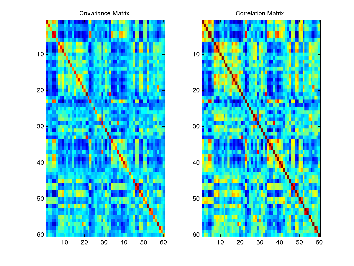
Why does it make sense that the data looks symmetric? Look to see which non-diagonal entry has the largest covariance. Look up the corresponding labels. Does it make sense that these two elements would have a high covariance? Compare with the largest non-diagonal correlation. Continue checking for the first TEN largest non-diagonal entries in the covariance and correlation matrices. You probably do not want to do this one by one. Instead create a loop to find the results. It may be useful to use Matlab's fprintf command to print out the results.
- Calculate the first principal component with the covariance and correlation matrices. The Matlab function eigs may be helpful to you. Visualize the elements of each using imagesc and compare your results. Your solution should look like this
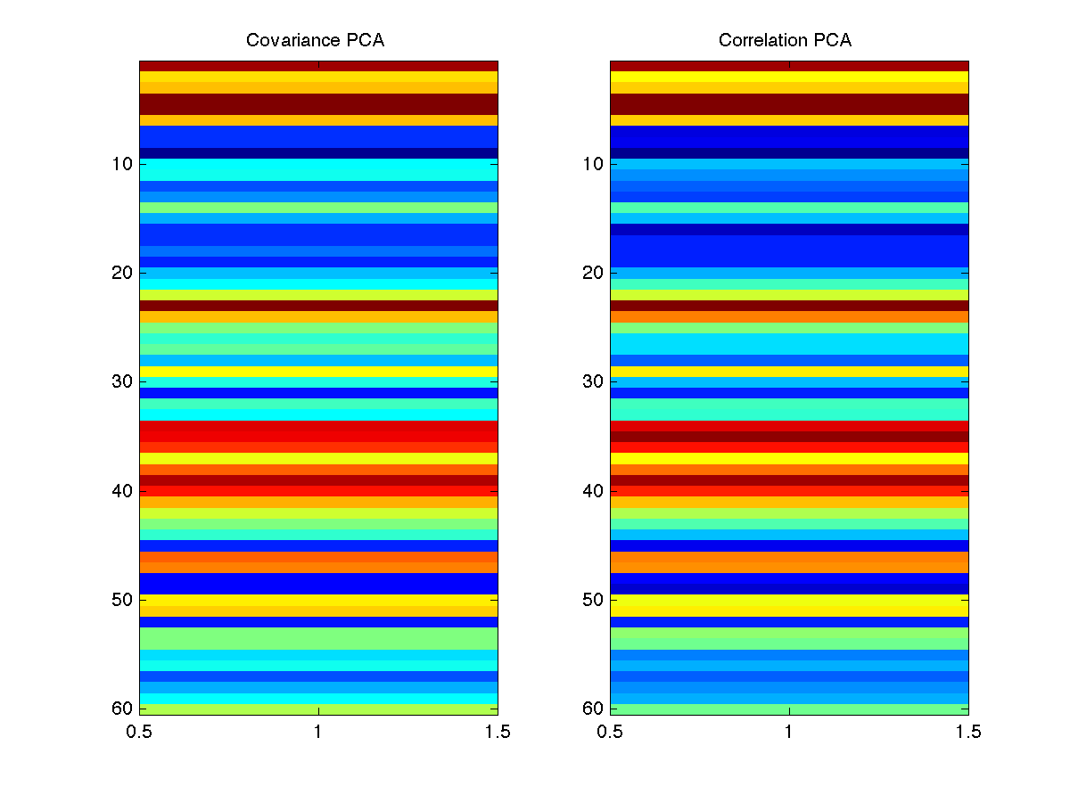
Use fprintf to compare the genres associated with the largest 10 elements of each principal component. Comment on the results.
- Post your m-file hw8Last.m to dropittome using the same password as we used in the first homework. In order to get full credit, your directories and files must be named correctly and you must have links to your function file and the m-file (script file) that created the webpage, along with the appropriate text, plots, and such to answer the problems.
|