|
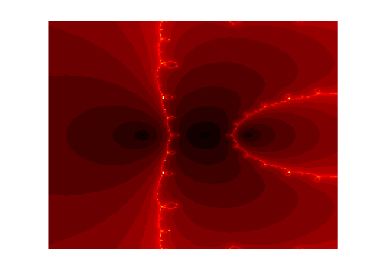
For this week's assignment, we will continue looking at functions and will use them to create pretty pictures such as the following:
 Complex Numbers
In order to create such pictures we need to review complex numbers and root finding techniques. Let's start with complex numbers. A complex number $z$ is defined in terms of two real numbers $a$ and $b$ such that
\[z = a+ib\]
Here $i$ is defined such that $i^2=-1$. Using this representation, many operations can be defined such as addition, multiplication, and division. For example, addition is defined as
\[z_1 + z_2 = (a_1 + a_2) + i (b_1+b_2)\]
and multiplication is defined as
\[z_1\times z_2 = (a_1a_2-b_1b_2) + i(a_1b_1 +a_2b_2)\]
In Matlab, a complex number can be defined in one of two ways
Note that the latter representation suggests that a complex number can be thought of as an ordered pair $(a,b)$. We will use this representation, in order to plot complex numbers where the real part is defined on the $x$ axis and the complex part is defined on the $y$ axis. Once a complex number is defined, you can just use the normal operations (+,-,/,*).
Calculating Roots
A root of a function $f(x)$ is defined as the points $x$ such that
\[f(x) = 0\]
For example, if
\[f(x)=x^2-4\]
then the roots are defined as $x=\pm 2$. In the last example, it was easy to find the roots using algebra. However, life can easily get difficult for more complicated problems. As a result, numerical methods are needed to come up with a solution.
Using the Taylor's series
\[f(x) = f(a) + f'(a)(x-a) + \frac{f''(a)}{2}(x-a)^2\ldots\]
we can create a method to find roots. Using just the first two terms of the series and using the assumption that $f(x)=0$ we see
\begin{eqnarray*}
0 &=& f(x) = f(a)+f'(a)(x-a)\\
f(a) &=&-f'(a)(x-a) \\
x &=& a -\frac{f(a)}{f'(a)}
\end{eqnarray*}
Thus we can define an iterative process to find roots where
\[\boxed{x_{k+1}=x_k -\frac{f(x_k)}{f'(x_k)}}\]
This process is known as the Newton's Method.
Subfunctions
In the last homework, we learned how to create functions. There can be many situations where it will be important to create subfunctions. For instance, you may want to have a main function that calculates the Newton's Method where $f$ and $f'$ are defined as subfunctions. This will be what you need to do for your homework. To build your intuition, consider the following Matlab m-file that consists of subfunctions:
function [f,fp]=subfun(x)
f = fun(x);
fp = derivFun(x);
end
function f = fun(x)
f = x.^2 + 2*exp(x);
end
function fp = derivFun(x)
fp = 2*x + 2*exp(x);
end
This is a simple m-file consisting of three subfunctions. The first one is called subfun that takes as input just the variable x and outputs f and fp. Here f is determined by the function fun and fp is defined by the function derivFun. They are all defined inside one m-file. Alternatively, these can be defined as different functions inside the same directory. Stylistically, there are pros and cons for each method. Can you think of some of the reasons to put the functions in one m-file verses multiple files?
Problem Set 6
- Create an m-file called hw6Last.m where Last is the first four letters of your last name in your MA302 folder. You should now have the tools to create your own published files by adapting your previous homework. Note that I will be grading format. Your published file should be polished as if you were to turn it in as a final report.
- Create an m-file newtLast.m that applies Newton's Method until $f(z)$ is below a predefined tolerance tol=1e-6. The function newtLast.m should take as an input z and returns the approximate root z and the number of iterations it needed to converge. Create two subfunctions f and fp in the same m-file that defines the function
\[f(z) = z^3 - 3^z\]
and its derivative, respectively. Calculate the number of iterations for Newton's Method to converge for the complex numbers with
- Real part: 200 equally spaced points between -5 and 8
- Complex part: 200 equally spaced points between -8 and 8
You may want to use the Matlab command meshgrid. Visualize the number of iterations per starting point z by using the Matlab command imagesc. You may want to change the colormap settings.
- If you take advantage of component-wise multiplication, Newton's Method can be ran on a vector of initial points. Run Newton's Method on the same function as above. However, the starting point is now a two dimensional vector where the
- x-values: 200 equally spaced points between -10 and 10
- y-values: 200 equally spaced points between -10 and 10
Can you explain why the solution looks like a bunch of squares? Can you explain why the solution looks differently than the solution from the last problem?
- Create a new m-file myNewtLast.m that runs Newton's Method on your own function with your own range of values. The values can be real or complex. Comment on the results.
- Post your m-file hw6Last.m to dropittome using the same password as we used in the first homework. In order to get full credit, your directories and files must be named correctly and you must have links to your function file and the m-file (script file) that created the webpage, along with the appropriate text, plots, and such to answer the problems.
|