|
For this assignment, I will be introducing you to Partial Differential Equations. If you enjoy this assignment, I encourage you to take Computational Methods next Fall. We will be interested in studying the wave equation:
\[\frac{\partial^2 h}{\partial t^2} = c^2 \frac{\partial^2 h}{\partial x^2}\]
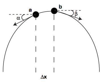
This equation comes up in numerous applications including oscillating strings. In order for you to get an intuition of where this equation comes from, imagine a taut string with an infintesimal distance $\Delta x$ between two points $a$ and $b$ on the string as shown below
 We make some assumptions on the string:
- The mass of the string $\rho$ is constant throughout
- The gravitational force on the string is ignored
- The string moves only in the vertical direction
With these assumptions, the motion on $a$ and $b$ can be represented with just the vertical components $T_a\sin\alpha$ and $T_b\sin\beta$. Thus, by Newton's Second Law
\begin{eqnarray*}
F &=& ma\\
T_b\sin\beta - T_a\sin\alpha &=& \rho\Delta x\frac{\partial^2 h}{\partial t^2}
\end{eqnarray*}
Now we are assuming that the string moves only in the vertical direction. Thus the horizontal motions must be constant. In other words
\[T_a\cos\alpha = T_b\cos\beta = T\]
Thus
\begin{eqnarray*}
\frac{T_b\sin\beta}{T_b\cos\beta} - \frac{T_a\sin\alpha}{T_a\cos\alpha} &=& \frac{\rho\Delta x}{T}\frac{\partial^2 h}{\partial t^2}\\
\tan\beta-\tan\alpha &=&\frac{\rho\Delta x}{T}\frac{\partial^2 h}{\partial t^2}
\end{eqnarray*}
But $\tan\alpha$ and $\tan\beta$ are the slopes of the string at $a$ and $b$ where $b = a+\Delta x$. Thus
\begin{eqnarray*}
\frac{1}{\Delta x}\left(\frac{\partial h}{\partial x}(a+\Delta x)-\frac{\partial h}{\partial x}(a)\right) &=&\frac{\rho}{T}\frac{\partial^2 h}{\partial t^2}
\end{eqnarray*}
If we now take the limit as $\Delta x\rightarrow 0$ we get
\[\boxed{\frac{\partial^2 h}{\partial t^2} = c^2 \frac{\partial^2 h}{\partial x^2}}\]
where $c^2 = \frac{T}{\rho}\ge 0$. This is an example of a Partial Differential Equation (PDE) as the derivatives are takes with respect to both time $t$ and horizontal space $x$. We are now interested in coming up with numerical methods to solve such problems.
In order for us to solve such problems, let's go back to our friend the Taylor's series
\[f(x+\Delta x) = f(x) + f'(x)\Delta x + \frac{f''(a)}{2}\Delta x^2\ldots\]
We assume $\Delta x$ is small so we can ignore higher order terms. Thus
\[f'(x) \approx \frac{f(x+\Delta x)-f(x)}{\Delta x}\]
We can also use this idea to approximate
\[f''(x) \approx \frac{f'(x) - f'(x-\Delta x)}{\Delta x} = \frac{\frac{f(x+\Delta x)-f(x)}{\Delta x} - \frac{f(x)-f(x-\Delta x)}{\Delta x}}{\Delta x} = \frac{f(x+\Delta x)-2f(x) + f(x-\Delta x)}{\Delta x^2} \]
This is known as the Central Difference approximation.
Now we can use this idea and extend it to partials:
\begin{eqnarray*}
\frac{\partial^2h}{\partial t^2} &=&\frac{h(x,t+\Delta t) - 2h(x,t) + h(x,t-\Delta t)}{\Delta t^2}\\
\frac{\partial^2h}{\partial x^2} &=&\frac{h(x+\Delta x, t) - 2h(x,t) + h(x-\Delta x, t)}{\Delta x^2}
\end{eqnarray*}
Plugging this into the wave equation
\begin{eqnarray*}
\frac{\partial^2 h}{\partial t^2} &=& c^2 \frac{\partial^2 h}{\partial x^2} \\
\frac{h(x,t+\Delta t) - 2h(x,t) + h(x,t-\Delta t)}{\Delta t^2}
&=&
c^2\frac{h(x+\Delta x, t) - 2h(x,t) + h(x-\Delta x, t)}{\Delta x^2}
\end{eqnarray*}
Thus
\[
h(x,t+\Delta t) = \frac{c^2\Delta t^2}{\Delta x^2}\left(h(x+\Delta x, t) - 2h(x,t) + h(x-\Delta x, t)\right) + 2h(x,t) - h(x,t-\Delta t)
\]
The goal for this assignment is to program this method.
In order to program this method, we need to create boundary conditions as the solution depends on both $x+\Delta x$ and $x-\Delta x$. In Matlab, since the first element of a vector is defined by 1, we assume that
\[2\le \textrm{xLoc}\le m-1\]
Then
\begin{eqnarray*}
\textrm{xLoc}=1&\Rightarrow&\textrm{left boundary condition}\\
\textrm{xLoc}=m&\Rightarrow&\textrm{right boundary condition}
\end{eqnarray*}
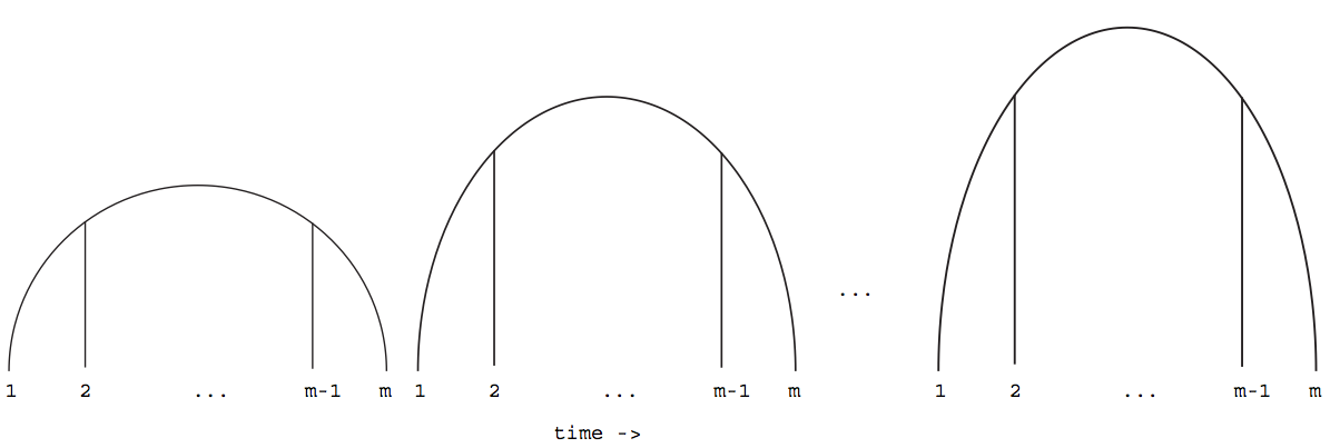
Note that here $\textrm{xLoc}=1$ corresponds to the left most point of a string and $\textrm{xLoc}=m$ corresponds to the right most point of a string. For an illustration consider
 At the end of the day, we can think of $h(x,t)$ as the matrix
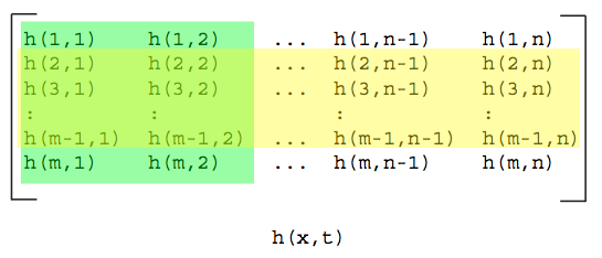 Notice the first and last row will depend on the boundary conditions (in yellow) and you will need the first two columns (in green) in order to tell what the function is doing in future time.
To simplify the process we will assume that our boundary conditions are 0 or
\[h(1,:) = h(m,:) = 0\]
and that the first timestep will equal the second timestep or
\[h(:,1) = h(:,2)\]
To summarize, the string of length $L$ will be split into sections $\Delta x$ where \[L = (m-1)\Delta x\]
and the total time $\textrm{totT}$ will be split into timesteps $\Delta t$ where
\[\textrm{totT} = (n-1)\Delta t\]
Problem Set 7
- Create an m-file called hw7Last.m where Last is the first four letters of your last name in your MA302 folder. A sample file is located here. For this assignment, I want you to include the animated GIF as well as your figures saved as png files. I will be grading format. Your published file should be polished as if you were to turn it in as a final report.
- Create a function stringLast.m that takes as input:
\begin{eqnarray*}
dx &=& \Delta x\\
dt &=& \Delta t\\
c2 &=& \frac{T}{\rho}\\
\textrm{L} &=& \textrm{Length of String}\\
\textrm{totT} &=& \textrm{Total Time of Simulation}
\end{eqnarray*}
and outputs the $m\times n$ matrix $h$ from above. Run stringLast.m with inputs (in the same order as outlined above):
>>h = stringLast(.1,.01,25,10,4);
Note that the initial height $h$ for the string should follow a smooth curve where it is of height 1 in the center and 0 at the ends.
- Create a new function animLast.m that takes as an input a string filename and matrix mat and creates an animated GIF of the columns of mat. Make sure your axes stay constant! It may be useful to use the animated GIF code from lecture 3. Apply this function on your matrix h from above. Your result will depend on what you chose to be your smooth curve. Example GIFs are:
- We will now illustrate Matlab's many methods for plotting. You could stack each timestamp of your h matrix to form a 3D graph using the built in Matlab command plot3. Next play with Matlab's built in functions mesh, contour, and imagesc. Note you can save your figures as png files using the Matlab command print. Don't forget to label each of your axes. Also, be sure to comment on the pros and cons of each method in your published file.
- BONUS: Change the boundary conditions to see other types of motions on the string.
- Post your m-file hw7Last.m to dropittome using the same password as we used in the first homework. In order to get full credit, your directories and files must be named correctly and you must have links to your function file and the m-file (script file) that created the webpage, along with the appropriate text, plots, and such to answer the problems.
|